Why F1 Score Fails on Imbalanced Datasets: MCC, PR-AUC, and the Limits of Harmonic Averaging
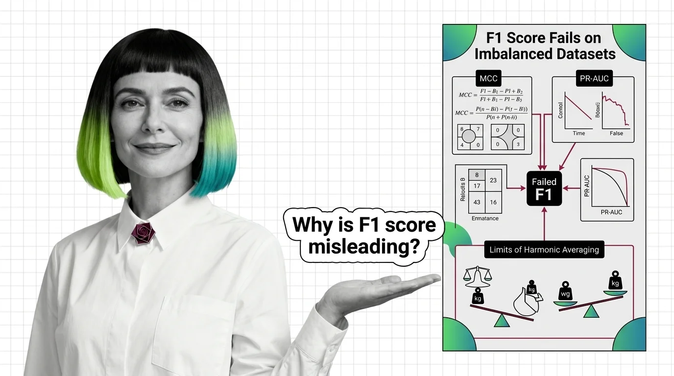
Table of Contents
ELI5
F1 score ignores true negatives — on imbalanced datasets, a useless classifier can score 0.95. MCC and PR-AUC read the full confusion matrix, exposing failures F1 hides.
A binary classifier scores an F1 of 0.95 on a medical dataset. The team validates against overfitting, runs cross-validation, presents results at a project review. The classifier has not identified a single negative case. On a dataset where 91% of instances belong to the positive class, predicting “positive” for everything earns a near-perfect F1 — while the Matthews Correlation Coefficient for the same classifier sits at -0.03 (Chicco & Jurman 2020). Worse than random. The metric that everyone checked said excellent. The metric that nobody checked said broken.
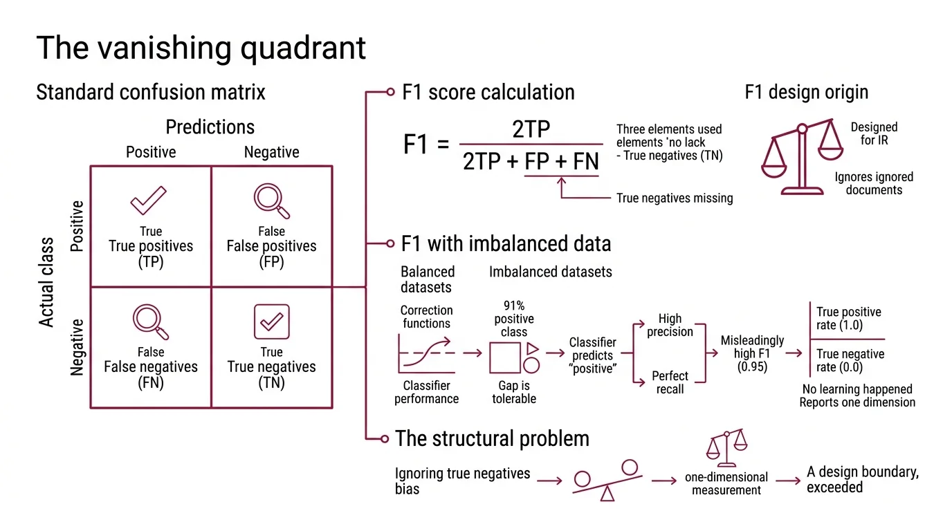
The Vanishing Quadrant
The Confusion Matrix is a two-by-two table: true positives, false positives, false negatives, true negatives. Four numbers that describe everything a binary classifier did. The Precision, Recall, and F1 Score uses only three of them.
F1 is defined as 2TP / (2TP + FP + FN) — a Harmonic Mean of precision and recall. True negatives are structurally absent from the formula. This is not an oversight; precision and recall were designed for information retrieval, where “correctly rejected irrelevant documents” was either infinite or undefined. In that original context, ignoring TN made perfect sense.
The problem arrives when you carry an information-retrieval metric into a classification problem where true negatives matter — which is most classification problems worth solving.
Why is F1 score misleading for imbalanced datasets
Think of F1 as a bathroom scale that only reads one of your feet. Shift your weight to the unmeasured foot and the number drops — not because you lost weight, but because the instrument was never designed to measure what you need.
On balanced datasets, this structural gap is tolerable. When positive and negative classes are equally represented, a classifier cannot score well on precision and recall while ignoring the negative class entirely — the math self-corrects through the denominator.
Class Imbalance removes that correction.
When 91% of samples are positive, a model that predicts “positive” for every input achieves high precision (most predictions happen to be correct) and perfect recall (no positives are missed). F1 combines these into 0.95. The classifier has learned nothing about distinguishing classes; it has learned that the majority label is a safe bet. The True Positive Rate is 1.0. The true negative rate is 0.0. F1 reports only the first number’s influence.
Not a bug. A design boundary, exceeded.
What a Correlation Coefficient Sees That a Harmonic Mean Cannot
Brian Matthews introduced the MCC in 1975 while studying protein secondary structure in T4 phage lysozyme (Matthews 1975). He needed a metric that treated predictions and observations symmetrically — one that would catch a model gaming the majority class. His solution was an adaptation of the phi coefficient applied directly to the confusion matrix.
The formula uses all four quadrants: MCC = (TP * TN - FP * FN) / sqrt((TP+FP)(TP+FN)(TN+FP)(TN+FN)). The range spans from -1 (perfect inverse prediction) through 0 (no better than random) to +1 (perfect prediction). A classifier that produces zero true negatives cannot achieve a high MCC — the TN term in the numerator collapses to zero, and the denominator factors involving TN ensure the score stays near or below zero regardless of how many positives the model captures.
F1 score vs Matthews correlation coefficient which metric is more reliable
The reliability question is not abstract. On the same 91%-positive dataset, the all-positive classifier scored F1 = 0.95 but MCC = -0.03 (Chicco & Jurman 2020). One metric says near-perfect; the other says slightly worse than coin-flipping.
MCC is more reliable because it is harder to game without genuine discrimination. F1 can be inflated by class distribution alone — predict the majority class and the harmonic mean rewards you. MCC cannot be inflated this way. A high MCC requires the classifier to perform well across all four quadrants of the confusion matrix, not just three.
There is a cost to this precision. MCC is less intuitive to interpret; its scale is not a probability, and its value depends on the marginal distributions of both classes. But the trade-off is stark: a metric that is easy to read and hides failures, versus a metric that is harder to read and does not.
For Model Evaluation on imbalanced problems — fraud detection, rare disease screening, anomaly identification — MCC is the structurally safer default.
Two Curves, Two Baselines, Two Stories
Single-number metrics compress classifier behavior into one point at one decision threshold. Curves preserve the full picture: performance across every possible threshold. But the two most common curves — ROC and precision-recall — disagree about what constitutes good performance on imbalanced data. The disagreement begins at the baseline.
When should you not use F1 score and use PR-AUC or ROC-AUC instead
ROC-AUC has a fixed random baseline of 0.5, regardless of class distribution. A random classifier on a 1%-positive dataset scores the same ROC-AUC as one on a 50%-positive dataset. This stability is reassuring — until it masks poor performance entirely. On the Hepatitis C dataset studied by Chicco and Jurman, a model achieved ROC-AUC of 0.8 while precision hovered near zero and MCC sat at +0.135 (Chicco & Jurman 2023). ROC said “good.” Every other metric disagreed.
PR-AUC anchors its baseline to the positive class prevalence — a random classifier scores an AUC equal to the prevalence rate (Saito & Rehmsmeier 2015). On a 1%-positive dataset, the random baseline is 0.01, not 0.5. This sensitivity is the point: the curve exposes exactly the region that matters most — how well the classifier handles the rare class, the class you built the model to find.
The practical recommendation depends on what you are measuring. Use PR-AUC when the cost of missing positives is high and the positive class is rare — medical screening, fraud detection, search relevance. Use ROC-AUC when both classes matter roughly equally and the dataset is reasonably balanced.
One caveat worth stating plainly: this recommendation is not universally settled. A 2024 study published in Patterns argues that ROC curves are robust to class imbalance, and that the perceived advantage of PR curves may reflect experimental design choices rather than a fundamental property of the metrics themselves. The debate remains open. The safest posture is to report both curves and let the disagreement surface rather than choosing one and trusting silence.
Only 12.1% of studies analyzing imbalanced datasets actually used PR curves in their evaluation (Saito & Rehmsmeier 2015). The majority relied on ROC or single-point metrics like F1 — the same metrics most likely to conceal the problems imbalanced data creates.
What the Missing Quadrant Predicts
If your dataset has pronounced class imbalance, F1 alone will overestimate model quality. The more extreme the imbalance, the wider the gap between the F1 score and actual discriminative ability. You can predict this from the formula: as the positive class dominates, precision’s denominator (TP + FP) shrinks relative to the true count, and recall approaches 1.0 for any model that defaults to the majority label.
If you switch from F1 to MCC on an existing evaluation pipeline, expect reported scores to drop — sometimes sharply. This does not mean your models got worse. It means your previous metric was not penalizing the failure modes that matter.
Both metrics are available in
Scikit Learn — f1_score and matthews_corrcoef sit in sklearn.metrics (scikit-learn Docs). The TunedThresholdClassifierCV class enables post-hoc threshold optimization, which becomes especially valuable when your target metric is MCC or PR-AUC rather than accuracy.
Rule of thumb: On any binary classification task where the minority class is substantially underrepresented, report MCC alongside — or instead of — F1. If you are comparing models across different datasets with different class distributions, MCC is the only standard single-number metric that accounts for all four confusion matrix entries.
When it breaks: MCC assumes a fixed confusion matrix at a single decision threshold. For probabilistic classifiers where you need to evaluate calibration and ranking across all thresholds, MCC alone is insufficient — pair it with PR-AUC. On multi-class problems, MCC’s interpretation becomes less straightforward; the binary intuition of “correlation between prediction and truth” does not extend cleanly to three or more classes without additional assumptions. And no metric — not MCC, not PR-AUC — survives Benchmark Contamination. If your test set’s class distribution differs from what the model will encounter in practice, every threshold-dependent metric will mislead.
The Data Says
F1 score is structurally blind to true negatives. On imbalanced datasets, this blindness produces scores that reward majority-class prediction as if it were genuine discrimination. MCC corrects for this by reading all four quadrants of the confusion matrix; PR-AUC addresses the threshold dimension by anchoring its baseline to class prevalence rather than a fixed 0.5. The fix is not choosing one metric — it is understanding which failure mode each metric cannot see.
AI-assisted content, human-reviewed. Images AI-generated. Editorial Standards · Our Editors