What Is Vector Indexing and How HNSW, IVF, and Product Quantization Make Nearest-Neighbor Search Fast
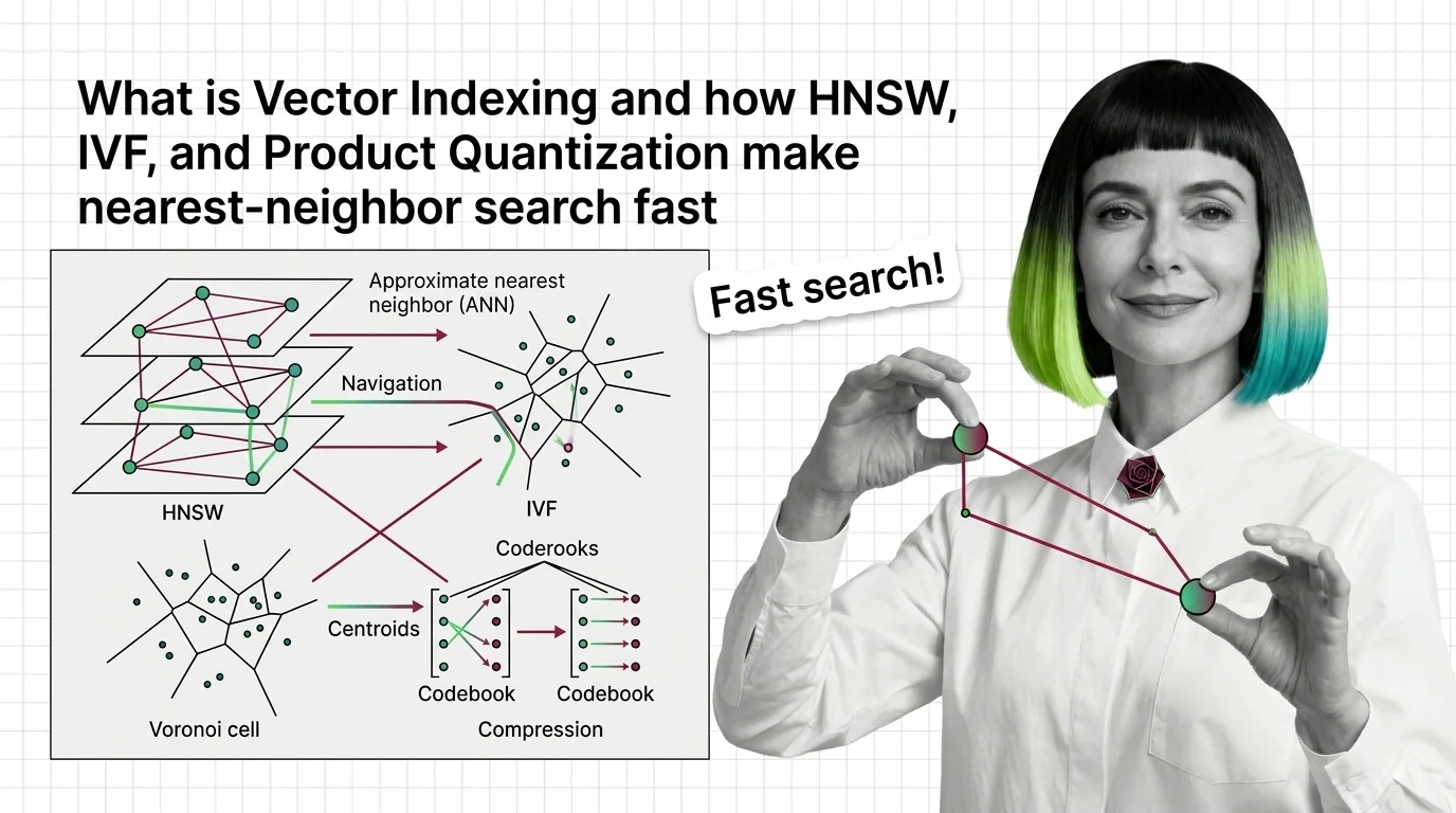
Table of Contents
ELI5
Vector indexing builds data structures — graphs, partitions, compressed codes — that let algorithms skip most vectors during search, trading a small accuracy loss for orders-of-magnitude speed gains in nearest-neighbor lookup.
A brute-force scan of one million 768-dimensional vectors takes roughly a second on modern hardware. The same query through an HNSW index returns in under a millisecond — a thousand times faster — and the answer is slightly wrong. Not catastrophically wrong. Deliberately, usefully wrong. That deliberate wrongness is the entire discipline of vector indexing, and the math behind it is more elegant than the name suggests.
The Geometry Problem Underneath Every Semantic Search
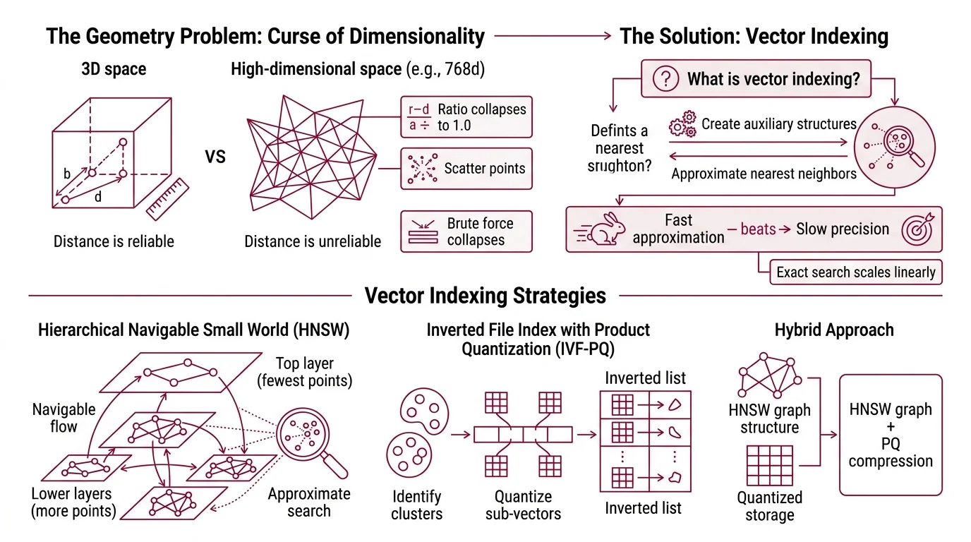
High-dimensional space behaves nothing like the three-dimensional world you navigate daily. In 768 dimensions — the Embedding size of many modern encoders — distance itself becomes unreliable. Points that appear “close” by one metric scatter apart by another; the ratio between the nearest and farthest point collapses toward 1.0 as dimensions grow. This is the curse of dimensionality, and it is the reason brute-force search strategies collapse at scale.
Vector indexing exists to make that collapse optional.
What is vector indexing in machine learning?
Vector indexing is the construction of auxiliary data structures over a collection of high-dimensional vectors so that Similarity Search Algorithms can locate approximate nearest neighbors without scanning the entire dataset. The “approximate” qualifier is not a concession — it is an engineering decision. Exact nearest-neighbor search scales linearly with dataset size: doubling your vectors doubles your latency. For a retrieval-augmented generation pipeline querying millions of embeddings at inference time, linear scaling is not slow. It is unusable.
Fast approximation beats slow precision — that is the core trade-off. Every vector index encodes a bet about which vectors can be safely ignored for a given query.
The three dominant strategies for making that bet are graph-based navigation (HNSW), space partitioning with compression (IVF with Product Quantization), and hybrid approaches that combine both. Each exploits a different geometric property of the data — and each fails differently when the geometry doesn’t cooperate.
How does HNSW build a navigable small world graph for approximate nearest neighbor search?
HNSW — Hierarchical Navigable Small World — treats the vector collection as a multi-layered graph. The idea, introduced by Malkov and Yashunin in a 2016 paper and published in IEEE TPAMI in 2018, borrows from network science: if you build a graph where most nodes connect to nearby neighbors but a few long-range links exist, greedy traversal converges quickly.
Picture a city with local streets and express highways. Searching for a destination starts on the highway layer — few nodes, long jumps, coarse navigation. At each layer, the algorithm greedily hops to whichever neighbor is closest to the query vector. When it can no longer improve, it drops one layer and continues with finer granularity until it reaches the bottom layer, where all vectors live and connections are dense.
The construction process assigns each new vector to layers probabilistically, using an exponentially decaying function — most vectors appear only on the bottom layer; a few propagate upward. This ensures the top layers stay sparse enough for fast traversal while the bottom retains full resolution.
The result is logarithmic search complexity (Malkov & Yashunin). A dataset of one million vectors requires roughly twenty hops; a billion vectors, roughly thirty. That logarithmic scaling is the reason HNSW dominates in-memory nearest-neighbor search across most benchmark conditions.
But graphs carry a cost. Every node stores its embedding plus its connections in RAM. For a billion 768-dimensional float32 vectors, the raw data alone consumes roughly three terabytes — before graph overhead. What happens when your hardware budget doesn’t stretch that far?
Slicing the Space: How Partitions and Compressed Codes Replace Brute Force
The alternative to navigating a graph is to never build one. Inverted File Index (IVF) combined with Product Quantization (PQ) takes a fundamentally different approach: partition the space, compress the vectors, and search only the relevant slices.
How does IVF with product quantization compress and partition vectors for fast retrieval?
IVF starts by clustering the vector collection using k-means. Each cluster centroid defines a Voronoi cell — a region of space where every point is closer to that centroid than to any other. At query time, the algorithm identifies the nearest centroids and searches only vectors assigned to those cells, ignoring the rest of the dataset entirely.
Product Quantization then compresses the vectors within each cell. The key insight from Jégou, Douze, and Schmid’s 2011 IEEE TPAMI paper is decomposition: split each high-dimensional vector into smaller subvectors — say, eight slices of a 768-dimensional vector, each slice covering 96 dimensions — and quantize each slice independently against a small codebook. Instead of storing the original float32 values, you store a sequence of codebook indices.
The compression is dramatic. A 768-dimensional float32 vector occupies 3,072 bytes. With PQ using 8 subquantizers and 256 centroids per subquantizer, the same vector compresses to 8 bytes — a compression ratio of 384 to one. Enough to keep a billion-vector index in tens of gigabytes rather than terabytes.
Not lossy storage. Strategic forgetting.
Distance computation shifts accordingly. Instead of computing exact distances to full-precision vectors, the algorithm uses precomputed lookup tables of distances between query subvectors and codebook centroids. This asymmetric distance computation (ADC) introduced in the same paper approximates true distances at a fraction of the computational cost (Jégou et al.).
The recall-speed trade-off depends on two tunable parameters: the number of cells probed at query time (nprobe) and the PQ codebook granularity. Neither has a universally correct value — both require tuning per dataset and recall target. Anyone who gives you a fixed nprobe number without knowing your data is guessing.
So which strategy should you use — graph or partition? That depends entirely on what you’re willing to sacrifice.
Four Strategies, Four Bets on Geometry
Vector indexing is not a single algorithm. It is a family of competing bets about how to exploit the structure of high-dimensional data.
What are the main types of vector index algorithms and how do they compare?
The four major families differ in what they precompute and what they sacrifice:
| Strategy | Core Idea | Strength | Cost |
|---|---|---|---|
| Flat (brute-force) | Compare query to every vector | Perfect recall — no approximation | Linear latency; unusable at scale |
| Graph-based (HNSW) | Multi-layer navigable graph with greedy traversal | Highest recall at low latency; logarithmic scaling | High memory — full vectors plus graph structure in RAM |
| Partition + compression (IVF-PQ) | Cluster vectors, compress with product quantization, search partitions | Massive compression; billions of vectors on modest hardware | Lower recall ceiling; requires careful parameter tuning |
| Disk-based hybrid ( DiskANN) | Graph navigation with SSD-resident vectors and in-memory compressed graph | Billion-scale on a single node with limited RAM | SSD latency on cache misses; graph build is slow |
DiskANN, introduced by Subramanya et al. at NeurIPS 2019, demonstrated billion-point search on a single machine with 64GB of RAM and an SSD — a feat that previously required distributed clusters (Microsoft Research). The project has since been rewritten in Rust; the legacy C++ codebase has moved to a separate branch and is no longer actively developed (DiskANN GitHub).
ScaNN, Google’s library, introduced the SOAR algorithm — Spilling with Orthogonality-Amplified Residuals — at NeurIPS 2023, which improves partitioned search accuracy by amplifying residual orthogonality to reduce quantization error without adding partitions (Google Research).
FAISS, Meta’s vector search library, remains the most widely adopted implementation. As of version 1.14.1, it supports flat, IVF, HNSW, PQ, residual quantization, and several hybrid index types (FAISS Docs). GPU acceleration via NVIDIA cuVS integration achieves up to 12.3x faster build times and 4.7x lower search latency compared to CPU HNSW (Meta Engineering).
No single algorithm dominates all conditions. ANN-Benchmarks, the standard evaluation suite, reflects this — leaderboard positions shift as new submissions arrive, and the relative ranking of algorithms depends heavily on dataset characteristics, recall targets, and hardware constraints.
Choosing Your Index by What It Sacrifices
The mechanism-level understanding above translates directly into engineering predictions.
If your dataset fits in RAM and you need high recall, graph-based indexing — HNSW or its variants — is likely the shortest path to acceptable latency. But memory consumption scales linearly with dataset size, and that scaling has no compression escape hatch within the graph structure itself.
If your dataset exceeds available memory, IVF-PQ or disk-based approaches become necessary. Every additional layer of compression introduces quantization error that erodes recall. The relationship is monotonic: more compression, lower recall ceiling.
If latency variance matters more than average latency — as it does in user-facing search — graph-based approaches tend to produce more predictable query times than partition-based methods, where a query landing near cell boundaries may trigger probes across many partitions.
Rule of thumb: Pick the index type by your binding constraint — memory, latency, or recall — not by default reputation.
When it breaks: All approximate indices share a failure mode: queries near the boundary of the data distribution — outliers, adversarial inputs, vectors from a domain shift — receive the weakest approximation guarantees. The vectors the index was designed to skip are precisely the ones the query needed. When retrieval accuracy drops on tail queries, the index structure itself is usually the first place to investigate.
The Data Says
Vector indexing is geometry management under constraints. HNSW bets on graph traversal and pays in memory; IVF-PQ bets on partitions and compression and pays in recall; DiskANN bets on SSD-backed graphs and pays in build time. Each strategy trades accuracy for speed along a different axis, and the right choice depends on dataset size, memory budget, and the recall floor your application can tolerate. There is no default.
AI-assisted content, human-reviewed. Images AI-generated. Editorial Standards · Our Editors