What Is Text-to-Speech AI and How Neural TTS Architectures Convert Text into Speech
ELI5
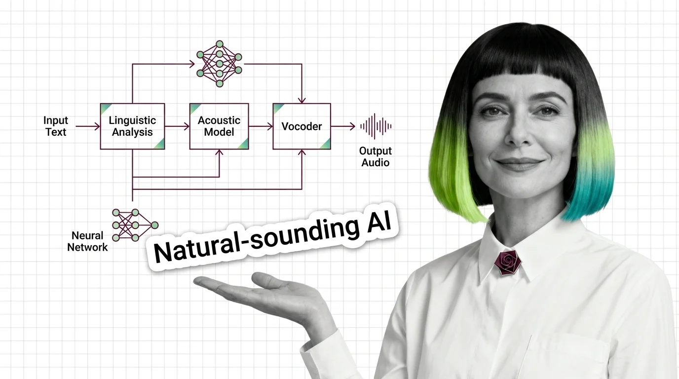
Text-to-speech AI converts written text into spoken audio using neural networks trained on thousands of hours of human speech — no handcrafted phoneme rules required. The model learns acoustic patterns end-to-end and synthesizes waveforms directly.
The gap between synthetic voice and human speech closed faster than the audio industry expected. When Tacotron 2 was presented at ICASSP 2018, it scored 4.53 on the Mean Opinion Score scale — professional human recordings averaged 4.58 (Tacotron 2 paper). The difference was smaller than the variation between individual speakers. For decades, text-to-speech was the domain of phoneticians who built explicit pronunciation dictionaries, hand-tuned prosody rules, and carefully spliced recorded phoneme units into waveforms. Then it wasn’t. The reason isn’t that compute became abundant. The reason is that the architecture changed entirely.
The old model was a pipeline: convert text into linguistic features, map those features to acoustic parameters through handcrafted rules, synthesize a waveform. Each stage required deep domain expertise. The new model replaces all three stages with a single learned function.
Not a faster pipeline.
A different kind of machine entirely.
From Rules to Learned Mappings
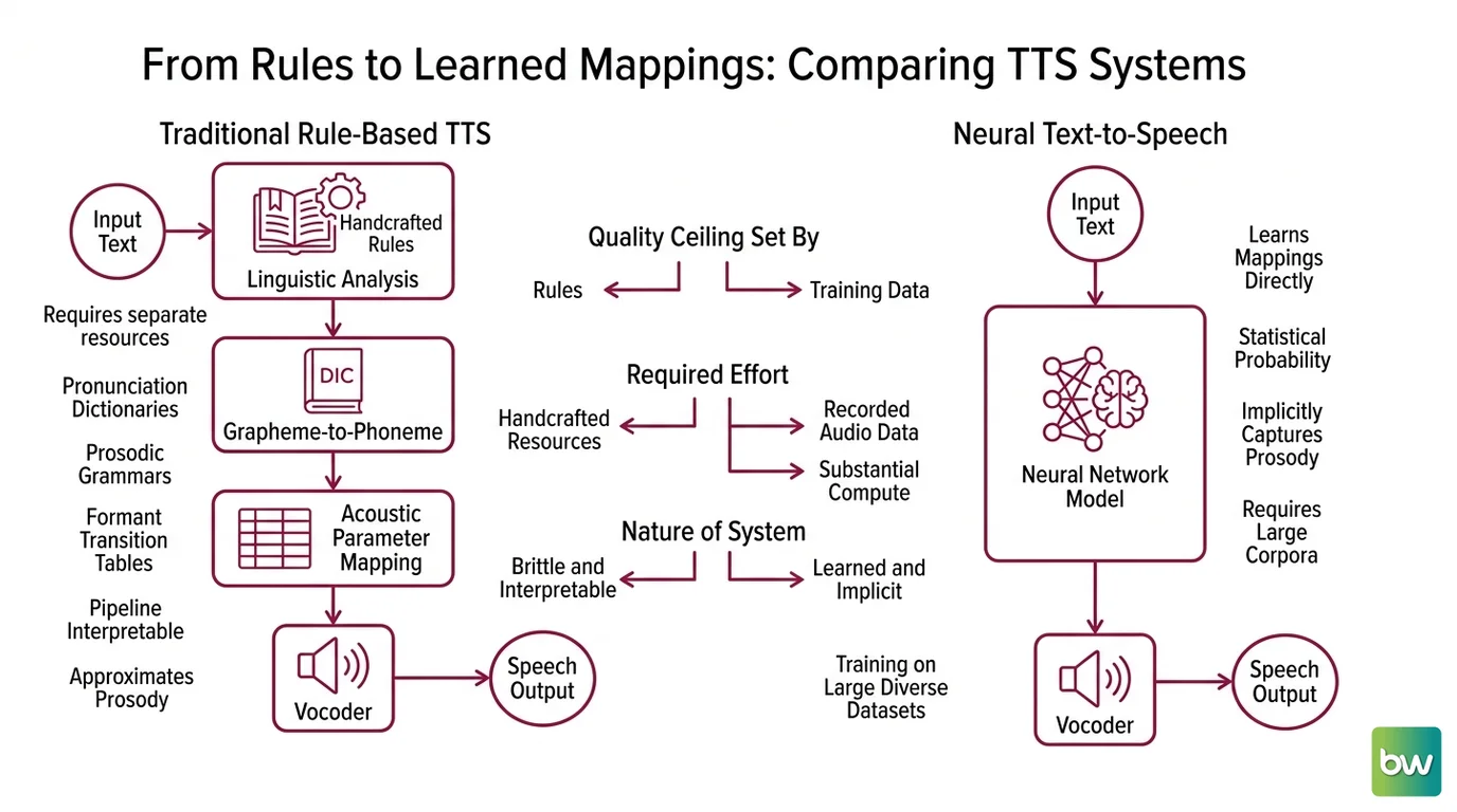
Rule-based TTS systems built their acoustic output from explicit linguistic knowledge — phoneme dictionaries, formant transition tables, prosodic grammars tuned by speech scientists. Each language required a separate set of handcrafted resources, and each new domain (medical terminology, legal language, proper names) required new entries. Neural TTS abandons that premise and learns the relationship between text and speech directly from recorded audio paired with transcripts. Training data, not rules, sets the quality ceiling — at the cost of requiring large corpora and substantial compute to reach that ceiling.
What is text-to-speech AI and how is it different from traditional rule-based TTS?
Traditional TTS operates on explicit linguistic rules. A text string is converted into Phoneme sequences — the atomic sound units of spoken language — using pronunciation dictionaries. Those sequences are then mapped to acoustic parameters through rule tables or statistical models, and a Vocoder converts the parameters to audio. This pipeline is interpretable; every decision is traceable to a specific rule or table entry. It is also brittle. Any word, name, or construction not covered by the dictionary produces mispronunciation, and prosody — the rhythm and intonation of natural speech — must be approximated by rules that cannot capture human-level variability.
Neural text-to-speech does not operate this way. Instead of converting text to phonemes via a dictionary, a neural model learns a statistical mapping from text (or intermediate phoneme representations) to acoustic output. This mapping is estimated from training data — typically thousands of hours of recorded speech paired with transcripts. The model learns which acoustic patterns correspond to which linguistic inputs, implicitly capturing both pronunciation and prosody. The explicit rule system is replaced by a probability distribution over acoustic outcomes, estimated from observed data rather than specified by experts.
The consequence is not merely better quality. It is a different failure mode. Rule-based systems fail predictably, on identifiable gap cases in their dictionaries. Neural systems fail stochastically, on inputs that fall outside their training distribution — a distinction that becomes important when diagnosing where these systems break in production.
How does a neural text-to-speech model convert written text into natural-sounding audio?
The architecture that first demonstrated near-human quality was Tacotron 2, developed at Google and presented at ICASSP 2018 (Tacotron 2 paper). It established the dominant paradigm for several years: a two-stage pipeline where the first stage predicts an intermediate acoustic representation and the second stage converts that representation to a waveform.
The intermediate representation is a Mel Spectrogram — a two-dimensional matrix that captures how audio energy is distributed across frequency bands over time. Predicting a mel spectrogram is computationally tractable in a way that predicting raw waveform samples is not; a mel spectrogram compresses seconds of audio into a manageable array, while raw waveforms require generating tens of thousands of sample values per second. The acoustic model focuses on what is linguistically meaningful, and a neural vocoder handles the high-frequency reconstruction from spectrum to waveform. Tacotron 2 used WaveNet as its vocoder; later systems moved to faster alternatives like HifiGAN, which produce comparable quality at a fraction of the compute cost.
The two-stage approach works well, but it introduces coupling between components. Errors in spectrogram prediction propagate into waveform quality, and the two models must be trained to work together. VITS (Conditional Variational Autoencoder with Adversarial Learning for Text-to-Speech, Kakao Enterprise, 2021) eliminated the separate mel stage by learning a direct mapping from text to a latent speech representation (VITS paper). VITS uses a variational autoencoder to encode speech into a latent distribution, normalizing flows to increase the expressiveness of that distribution, and adversarial training to refine the resulting waveform quality. A stochastic duration predictor allows the model to produce natural variation in speaking rate, rather than a rigid mapping of phonemes to fixed durations — which is one reason VITS-based systems sound less mechanically paced than two-stage predecessors.
More recent architectures apply flow matching to the generation problem. F5-TTS (2025) uses a diffusion transformer that generates audio fully non-autoregressively, reaching a real-time factor of 0.15 — producing a second of audio in 150ms of compute — without requiring explicit phoneme alignment during inference (F5-TTS paper). The architectural trajectory across these systems is consistent: fewer handcrafted intermediate representations, more learned mappings from observed speech data.
Inside the Stack: Components of a Modern Neural TTS System
Architecture choices determine the quality ceiling, but the engineering subproblems that remain constant across architectures determine whether a model handles production inputs correctly. Every neural TTS system — whether two-stage, end-to-end variational, or flow-matching — must solve the same set of problems.
What are the main components of a modern neural TTS system?
Text normalization handles the gap between written and spoken language: expanding “Dr. Smith” into “Doctor Smith,” reading numerical sequences in context, disambiguating abbreviations, handling URLs, currency, and code identifiers. This stage remains largely rule-based in production systems — not because neural approaches cannot handle it in principle, but because the tail cases are too consequential to leave to statistical inference. A system that mispronounces a medication name during a medical consultation, or renders a financial figure incorrectly in an earnings summary, fails in ways that are immediately visible and difficult to remediate.
The acoustic model is where architectural choices matter most. In two-stage systems, this component predicts a mel spectrogram using an encoder-decoder architecture with attention. In end-to-end systems, it learns a direct mapping to a latent speech representation. Duration modeling — deciding how long each phoneme or linguistic unit lasts — is either explicit (a separate duration predictor, as in VITS’s stochastic duration predictor) or implicit (learned through attention weights, as in the original Tacotron). Duration modeling quality is one of the primary variables separating natural-sounding speech from speech that sounds mechanically timed.
The vocoder converts spectral or latent representations to audible waveforms. Neural vocoders — HifiGAN and its derivatives — are now the production standard. They produce high-fidelity waveforms at a fraction of the compute cost of WaveNet, which required autoregressive sample-by-sample generation that was too slow for real-time deployment. Fast vocoder inference is what makes streaming TTS possible in interactive applications.
Voice conditioning allows modern systems to produce multiple speakers, styles, or emotional registers from a single model. ElevenLabs Eleven v3 (70+ languages, emotionally expressive, optimized for audiobooks and narration) encodes a speaker embedding from a short reference audio clip, conditioning the acoustic model to match the target voice (ElevenLabs Docs). Fish Audio S2-Pro (4B parameters, open-sourced March 2026) supports thousands of natural-language emotion tags for fine-grained prosody control and achieves a word error rate of 0.54% on Chinese and 0.99% on English — the lowest among all evaluated systems including proprietary ones (Fish Audio S2 paper). Cartesia Sonic 3.5 achieves sub-90ms end-to-end latency across 42 languages, optimized for real-time conversational agents (Cartesia Docs).
On the open-weight end,
Kokoro TTS (82M parameters, Apache 2.0, 8 languages) is designed for CPU inference — genuine on-device deployment without GPU dependency (Kokoro HuggingFace).
XTTS v2 supports voice cloning from a short reference clip across more than a dozen languages, though Coqui AI shut down in January 2024; the community coqui-tts fork on PyPI remains active, but no new model training is planned.
Compatibility notes:
- ElevenLabs deprecated models (eleven_monolingual_v1, eleven_multilingual_v1, eleven_turbo_v2, eleven_turbo_v2_5): Removed as of July 9, 2026. Migrate to Eleven v3 or Flash v2.5 (ElevenLabs Docs).
- XTTS v2: Coqui AI shut down January 2024; the
coqui-ai/TTSGitHub repo is no longer officially maintained. Use the community forkcoqui-ttson PyPI.- Cartesia T2A API: Deprecated in 2026. PVC model routing now requires dated model IDs (e.g.,
sonic-3-2026-01-12) per Cartesia changelog.
What the Architecture Predicts — and Where It Breaks
The shift from handcrafted rules to learned mappings makes specific predictions about failure modes. These are not edge cases; they are structural consequences of how the system was built.
If the text you send a neural TTS model closely resembles its training distribution — natural conversational speech, narrative prose, common proper nouns — output quality is high. If the text diverges from that distribution — programming identifiers, mathematical notation, domain-specific abbreviations, rare languages or dialects — the model generates a phonetically plausible but semantically incorrect rendering. The effect is reproducible. The remedy is not a larger model or different architecture; it is a text normalization layer that converts out-of-distribution input into forms the model was trained on.
If you need sub-100ms latency for real-time agent applications, streaming-optimized models are the correct architectural choice: Cartesia Sonic 3.5 at sub-90ms, ElevenLabs Flash v2.5 at approximately 75ms across 32 languages (ElevenLabs Docs). Fish Audio S2-Pro’s superior benchmark accuracy comes with infrastructure requirements incompatible with real-time streaming — quality scales; latency punishes size — in most deployment environments.
If you need local or on-device deployment without GPU access, Kokoro-82M's lightweight architecture makes it the realistic option; the multi-billion-parameter models require memory budgets that most edge environments cannot satisfy.
Rule of thumb: choose a model whose training data matches your deployment context in domain, language, and speaking style. The gap between training distribution and production input determines failure frequency more reliably than benchmark scores.
When it breaks: neural TTS systems fail consistently on out-of-distribution inputs — unusual proper nouns, programming identifiers, mathematical expressions, and languages with sparse training data. This is not a fixable engineering bug. It is a property of statistical mappings: they cannot generalize to patterns outside their training distribution, regardless of model size or architecture. Text normalization preprocessing addresses this more effectively than model substitution.
Two additional constraints require explicit review before production use. Fish Audio S2-Pro is published under a FISH AUDIO RESEARCH LICENSE — not a standard open-source license; commercial use requires a separate review before deployment. Kokoro-82M’s training data includes synthetic audio from commercial TTS providers, which may carry downstream licensing implications (Kokoro HuggingFace).
The Data Says
Neural text-to-speech replaced rule-based synthesis because end-to-end learned mappings capture naturalness that no finite set of handcrafted phoneme rules could produce. Tacotron 2 scored 4.53 MOS at ICASSP 2018 — within 0.05 of professional recordings (Tacotron 2 paper); current systems have extended that quality advantage into real-time latency, multilingual coverage, and voice adaptation from seconds of reference audio. The mechanism is statistical: the model encodes a probability distribution over acoustic outcomes given text inputs, and the training data defines the boundaries of that distribution as precisely as any rule system ever did — only the distribution is learned, not written.
AI-assisted content, human-reviewed. Images AI-generated. Editorial Standards · Our Editors