What Is Precision, Recall, and F1 Score and How the Confusion Matrix Drives Classification Evaluation

A classifier with 99% accuracy sounds like a triumph. Until you learn it was screening for a disease that affects 1% of the population and achieved that score by predicting “healthy” for every single patient. Every sick person missed. Every metric on the dashboard green. That gap between a comforting number and a dangerous reality is exactly what precision, recall, and the Confusion Matrix were built to expose.

The Four Cells Behind Every Classification Verdict

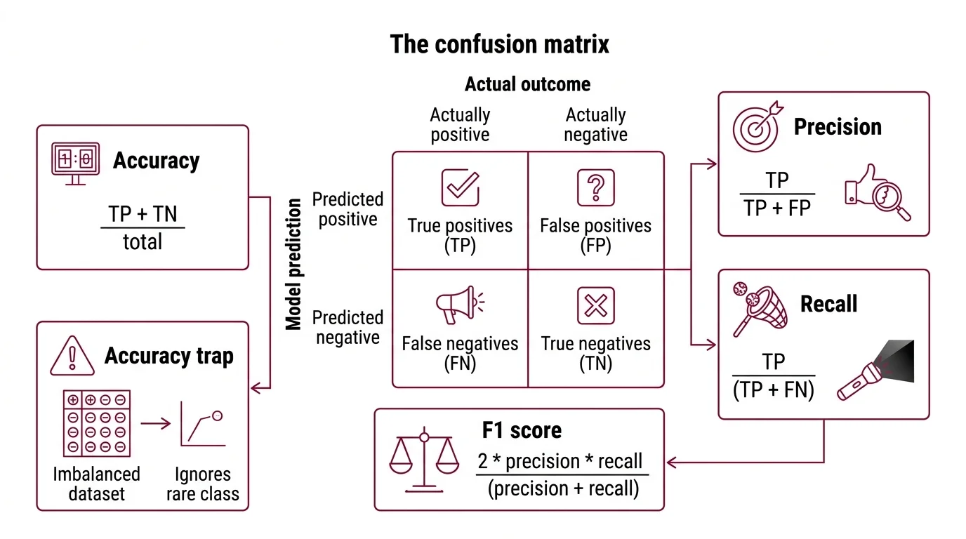
Every binary classifier produces four possible outcomes, and those four outcomes form a 2x2 grid — the confusion matrix. Rows represent what the model predicted; columns represent what actually happened. The entire field of Model Evaluation for classification traces back to reading that grid correctly.

What is precision recall and F1 score in machine learning

The four cells: true positives (TP) — the model said “yes” and was right. True negatives (TN) — the model said “no” and was right. False positives (FP) — the model said “yes” but was wrong. False negatives (FN) — the model said “no” but was wrong.

Accuracy counts how many predictions were correct out of all predictions: (TP + TN) / total. And here is the trap. In an imbalanced dataset — where one class vastly outnumbers the other — accuracy rewards a model for ignoring the rare class. A fraud detector that never flags fraud achieves 99.8% accuracy if only 0.2% of transactions are fraudulent.

The confusion matrix does not let you hide behind aggregates.

Precision = TP / (TP + FP). Of everything the model labeled positive, how much was actually positive? Precision punishes false alarms. If your spam filter sends important emails to junk, precision is low. High precision means: when this model says “yes,” you can trust it (Google ML Crash Course).

Recall = TP / (TP + FN). Of everything that was actually positive, how much did the model catch? Recall punishes misses. If your cancer screening fails to flag a tumor, recall is low. High recall means: this model does not let real positives slip through (Google ML Crash Course).

F1 score = 2 * precision * recall / (precision + recall). It compresses both metrics into a single value between 0 and 1 using the Harmonic Mean (Wikipedia). The name traces back to Van Rijsbergen’s Information Retrieval (1979), and was formally introduced at the MUC-4 conference in 1992 (Wikipedia).

Neither precision nor recall alone tells you whether a classifier is reliable. A model that labels everything as positive achieves perfect recall — and terrible precision. A model that labels only one supremely confident case as positive achieves perfect precision — and terrible recall. F1 forces both numbers to be decent before the score climbs.

How the Harmonic Mean Punishes Asymmetry

The choice of the harmonic mean is not arbitrary. It is the mechanism that gives F1 its diagnostic power — and understanding why requires seeing what happens when you use the wrong average.

How does the F1 score combine precision and recall using the harmonic mean

The arithmetic mean of 0.95 and 0.10 is 0.525 — a respectable-sounding number for a classifier with near-useless recall. The harmonic mean of the same pair is approximately 0.18.

That difference is the entire point.

The harmonic mean of two values is defined as 2ab / (a + b). Equivalently, F1 satisfies the relationship: 1/F1 = (1/2)(1/precision + 1/recall) (Wikipedia). The reciprocal form reveals the geometry: the harmonic mean operates in the space of rates, not magnitudes. A low value in either dimension drags the result down disproportionately — there is no hiding a weak metric behind a strong one.

This property makes F1 a conservative score. It rewards balance over extremes. If precision is 0.90 and recall is 0.90, F1 is 0.90. If precision is 0.99 and recall is 0.50, F1 drops to 0.665. The arithmetic mean would report 0.745 — a number that obscures the fact that half of all positive cases are being missed.

The general form, F-beta, introduces a parameter that controls the weighting: F-beta = (1 + beta squared) * precision * recall / (beta squared * precision + recall) (Wikipedia). When beta = 1, precision and recall carry equal weight — that is F1. When beta = 2, recall is weighted four times more heavily; useful in medical screening where missing a case is worse than a false alarm. When beta = 0.5, precision dominates.

Not a single formula. A family of tradeoff dials.

The Invisible Dial That Reshapes Every Metric

Most classifiers do not output a binary label directly. They output a probability score — and somewhere between that score and the final “positive” or “negative” label sits a Classification Threshold. Moving that threshold reshapes precision, recall, and F1 simultaneously.

How does the precision recall tradeoff work when you change the classification threshold

Picture a fraud detection model that assigns each transaction a score between 0 and 1. At a moderate threshold, anything above it gets flagged as fraud. Lower the threshold, and the model flags more transactions — catching more real fraud (recall rises) but also flagging more legitimate transactions (precision falls). Raise it, and the model becomes conservative — fewer false alarms (precision rises) but more real fraud slips through (recall falls).

This is the precision-recall tradeoff, and it is inescapable (Google ML Crash Course). You cannot improve both simultaneously by adjusting the threshold alone. The tradeoff is not a bug in the metric; it reflects a fundamental constraint in how probability scores map to binary decisions.

The threshold encodes a cost judgment. When false negatives are more expensive than false positives — medical screening, safety-critical systems — you lower the threshold and accept more false alarms. When false positives are more expensive — spam filtering, content moderation at scale — you raise the threshold and accept more misses (Google ML Crash Course).

F1 is what you get when you declare those costs equal. Which is also why F1 is sometimes the wrong metric.

The Roc Auc curve evaluates a classifier across all possible thresholds, providing a threshold-independent view of separability — a complementary lens to the single-threshold snapshot that F1 offers.

Where the Numbers Stop and the Decisions Start

If you change the class distribution in your test set, F1 changes — even if the model has not changed. If you evaluate on a dataset contaminated by training examples, F1 lies to you with a straight face. Benchmark Contamination is the silent failure mode of every leaderboard metric, F1 included.

If your task has severe class imbalance and you care about both positive and negative predictions, F1 has a structural blind spot: it ignores true negatives entirely. The Matthews Correlation Coefficient uses all four quadrants of the confusion matrix and is considered more informative for imbalanced data (Wikipedia). F1 and MCC answer different questions — F1 asks “how well does this model find positives?” while MCC asks “how well do this model’s predictions correlate with reality across all classes?”

If you are working with Scikit Learn, sklearn.metrics.f1_score supports five averaging modes: binary, micro, macro, weighted, and samples (scikit-learn Docs). Macro averaging treats each class equally; weighted averaging accounts for class imbalance. The choice of averaging mode can shift your F1 substantially on the same model — a detail that is rarely mentioned in benchmark comparisons.

Rule of thumb: If false positives and false negatives carry roughly equal cost, F1 is a reasonable single metric. If they do not — and they usually do not in production — use F1 as a starting point but make the cost asymmetry explicit through F-beta or a custom loss function.

When it breaks: F1 collapses as a reliable signal when the positive class is extremely rare and the evaluation set is small. With too few positive examples, a single additional false positive or false negative swings F1 by several points — making the metric unstable and comparisons between models unreliable.

The Data Says

The confusion matrix is not a report card. It is a diagnostic instrument — one that precision, recall, and F1 read from different angles. Accuracy hides the failure modes that matter most; the harmonic mean refuses to let one strong number compensate for one weak one. The metric you choose is a statement about which errors you can afford.