What Is Mixture of Experts and How Sparse Gating Routes Inputs to Specialized Sub-Networks
ELI5
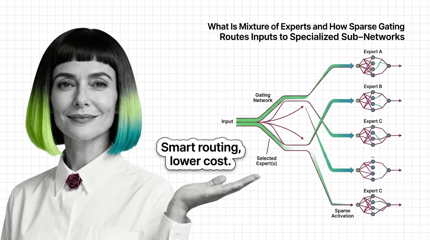
A mixture of experts model divides its neural network into specialized sub-networks and uses a learned gate to activate only the relevant few per input — storing vast knowledge while keeping compute costs low.
DeepSeek-V3 contains 671 billion parameters. On any given token, it activates roughly 37 billion of them. The remaining 94% are architecturally present but computationally silent — not broken, not wasted, but deliberately offline. That ratio tells you more about how modern language models actually scale than any benchmark leaderboard.
The Network That Mostly Stays Quiet
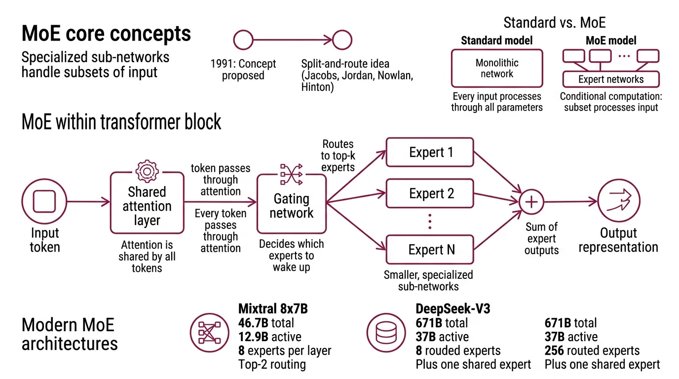
A standard transformer pushes every input through every parameter in every layer. Mixture of experts does something structurally different: it replaces the monolithic feed-forward network within each transformer block with a collection of smaller, specialized sub-networks — the “experts” — and inserts a trainable gate that decides which ones to wake up for each token.
The concept is older than most people assume. Jacobs, Jordan, Nowlan, and Hinton proposed the split-and-route idea in 1991 — over two decades before the transformer architecture existed.
What is mixture of experts in AI?
Mixture of experts (MoE) is a neural network architecture where input is processed by a subset of specialized sub-networks rather than the full model. The original 1991 formulation divided a complex problem space into regions, each handled by a dedicated “expert” — a small network trained to excel in its assigned territory — while a gating function learned how to assign inputs to the right expert.
In modern Inference pipelines, MoE operates inside the transformer. The self-attention layers remain shared; every token passes through the same attention mechanism. But the feed-forward layers — which typically account for roughly two-thirds of a transformer’s parameters — are replaced by N parallel expert networks. A gating network examines each token’s hidden representation and routes it to a small number of those experts.
The result is conditional computation. The model’s total parameter count reflects its stored knowledge; the active parameter count reflects the cost of any single forward pass. Mixtral 8x7B, for instance, holds 46.7 billion total parameters but activates only 12.9 billion per token — eight experts per layer with top-2 routing (Mistral AI Blog). DeepSeek-V3 pushes the ratio further: 671 billion total, 37 billion active, across 256 routed experts plus one shared expert per layer (DeepSeek-V3 Paper). Llama 4 Maverick continues the pattern at ~400 billion total with just 17 billion active, using 128 routed experts and top-1 routing (Meta AI Blog).
Not bigger networks. Selectively bigger networks.
How does the gating network in mixture of experts decide which expert to activate?
The gate is a learned linear layer followed by a softmax — simple in architecture, subtle in consequence.
Given an input token representation x, the gating network computes scores across all N experts. The formulation introduced by Shazeer et al. in 2017 adds tunable Gaussian noise to those scores before applying softmax, a technique called noisy Top K Routing. The noise encourages exploration during training: without it, the gate tends to collapse, sending all tokens to the same handful of experts while the rest atrophy from disuse.
The formal expression is clean: G(x) = Softmax(KeepTopK(H(x), k)), where H(x) includes the noise term and KeepTopK zeroes out all but the top-k scoring experts (Shazeer et al.). If k = 2, each token activates exactly two experts and the final output is a weighted blend of their responses. If k = 1, as in the Switch Transformer, each token sees exactly one expert — a binary routing decision with no blending.
That choice of k determines the tension between capacity and cost. Top-2 routing gives the model a richer representation per token but doubles the computation relative to top-1. Switch Transformers demonstrated that top-1 routing, despite its apparent crudeness, scaled to 1.6 trillion parameters across 2,048 experts and achieved a 4x pre-training speedup over T5-XXL (Fedus et al.). The original Shazeer et al. architecture achieved a capacity gain exceeding 1,000x with the noisy top-k approach — a ratio between total parameters and computational budget that dense models cannot match.
But routing alone creates a stability problem. Left unconstrained, the gate develops preferences — some experts become popular, others go unused, and the model’s effective capacity shrinks to a fraction of its theoretical capacity. This is where Load Balancing Loss enters: an auxiliary loss term that penalizes uneven token distribution across experts. The loss encourages the gate to spread tokens roughly equally, ensuring all experts receive training signal and develop distinct specializations rather than converging into redundant copies.
The gate is not just a router. It is a constraint surface — shaping which regions of the network learn what, and how evenly the model distributes its knowledge across its available capacity.
The Arithmetic of Selective Silence
The computational argument for MoE is almost embarrassingly direct. But the savings only materialize under a specific structural condition — and violating that condition is the most common source of disappointment with sparse architectures.
How does sparse activation in MoE reduce inference cost compared to dense models?
In a dense transformer, every token’s forward pass touches every parameter. The floating-point operations (FLOPs) per token scale linearly with the parameter count P. Double the parameters, double the cost per token.
MoE breaks that linear relationship. Because only k out of N experts activate per token, the FLOPs per token scale with the active parameter count — not the total. A model with 671 billion total parameters and 37 billion active costs roughly the same per forward pass as a dense 37-billion-parameter model, while storing the knowledge capacity of something far larger.
The practical implications are visible in the hardware. Expert Parallelism distributes different experts across different accelerators; since only a subset activates per token, the idle accelerators simply wait while the active ones complete their computation and return results. Google’s GLaM — 1.2 trillion parameters across 64 experts with top-2 routing — matched GPT-3’s quality benchmarks while consuming roughly one-third the training energy. The same principle applies at inference: you pay compute proportional to what you activate, not what you store.
The cost scales with what you use, not what you know.
Think of a dense model as a specialist who reads every book in the library before answering any question. An MoE model is a department — many specialists, one receptionist. The receptionist examines each question and routes it to two or three relevant experts. The library is just as large, but the labor per question is a fraction of the total headcount.
The catch — and it is a significant one — is memory. Every expert’s weights must be loaded or at least addressable, even when most remain inactive for any given token. An MoE model’s memory footprint scales with total parameters, not active parameters. For inference on limited hardware, this creates an asymmetry: you pay the memory cost of the full model but only the compute cost of the active slice. That asymmetry explains why MoE models often require distributed inference setups even when their active parameter count suggests a single GPU should suffice.
What the Routing Map Reveals
If every token in your input activates the same two experts, you have a load-balancing problem — the model has learned to route everything through its favorites, and most of its parameters contribute nothing. If the routing map shows diverse activation patterns across different input types, the model is using its capacity as intended: different regions of input space activate different combinations of expertise.
This observation has direct engineering consequences.
If you fine-tune an MoE model on a narrow domain, expect expert collapse. The gate will converge on the few experts most relevant to that domain while the rest receive no gradient signal. The effective model shrinks to a fraction of its nominal size. Broad generality requires training data broad enough to keep all experts alive and learning distinct functions.
If you increase the number of experts without increasing data volume proportionally, expect diminishing returns. More experts mean finer-grained specialization — but only if each expert receives enough training examples to specialize meaningfully. Under-provisioned experts learn nothing distinctive; they degrade into noisy copies of their neighbors and add memory cost without adding capability.
If you need deterministic outputs — identical results given identical inputs and seeds — MoE routing introduces a complication. Expert assignment can vary across batch compositions when using dynamic capacity factors, and in State Space Model hybrids that combine MoE with alternative sequence-processing layers, the interaction between routing decisions and state propagation remains an active research area with no settled best practice.
Rule of thumb: When total parameters vastly exceed active parameters, audit your expert utilization before scaling further — unused experts are expensive memory that produces no intelligence.
When it breaks: Load imbalance is the primary failure mode. If the gate consistently under-routes certain experts, those experts stop learning, the model’s effective capacity drops, and you pay the memory cost of a large model while receiving the quality of a small one. Auxiliary loss helps, but the balancing act introduces its own distortions. DeepSeek-V3’s adoption of auxiliary-loss-free load balancing (DeepSeek-V3 Paper) suggests the standard penalty was overriding quality-sensitive routing decisions — a fix that partially undermines the objective it was designed to protect.
The Data Says
Mixture of experts has moved from research curiosity to default architecture. As of 2025-2026, more than 60% of open-source AI model releases use MoE (NVIDIA Blog), and the reason is structural rather than fashionable: sparse activation is currently the only proven method for scaling total parameter count without proportionally scaling inference cost. The mechanism is efficient by arithmetic, not by accident.
AI-assisted content, human-reviewed. Images AI-generated. Editorial Standards · Our Editors