What Is Metadata Filtering and How It Constrains Vector Search Beyond Semantic Similarity
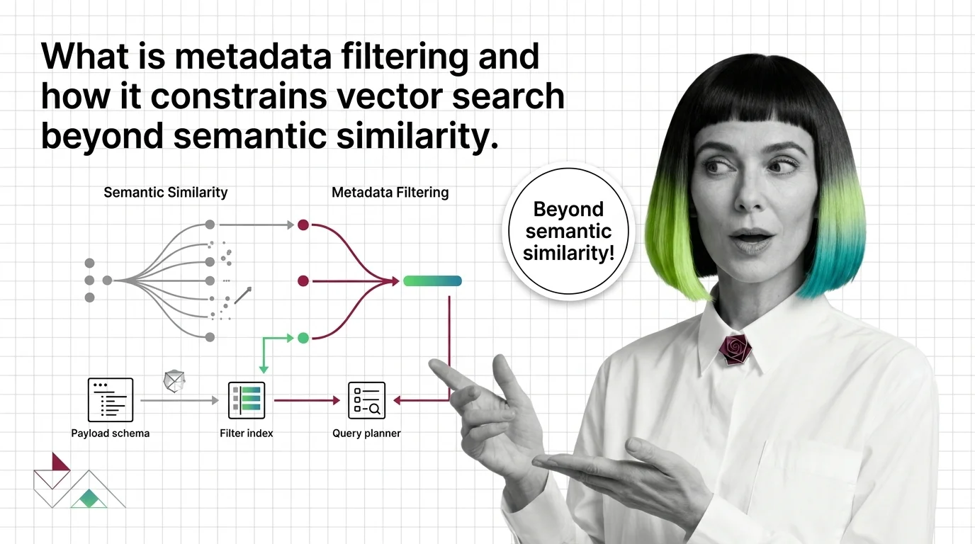
Table of Contents
ELI5
Metadata filtering attaches structured tags — tenant_id, language, published_after — to each vector, so the engine only considers points whose tags match a query’s predicates. Semantic similarity decides closeness; metadata decides what is allowed.
A vector database returns the most semantically similar chunk it knows about. That is the job. The problem appears the moment you ask it to be similar and also belong to the right tenant, the right language, and a date range that exists. The cosine score has no opinion about any of that. It will happily hand you a perfectly relevant document — written in the wrong language, owned by another customer, three years out of date. The fix is not better embeddings. It is a second axis of constraint, layered over the first.
What Vector Search Forgets, Metadata Filtering Remembers
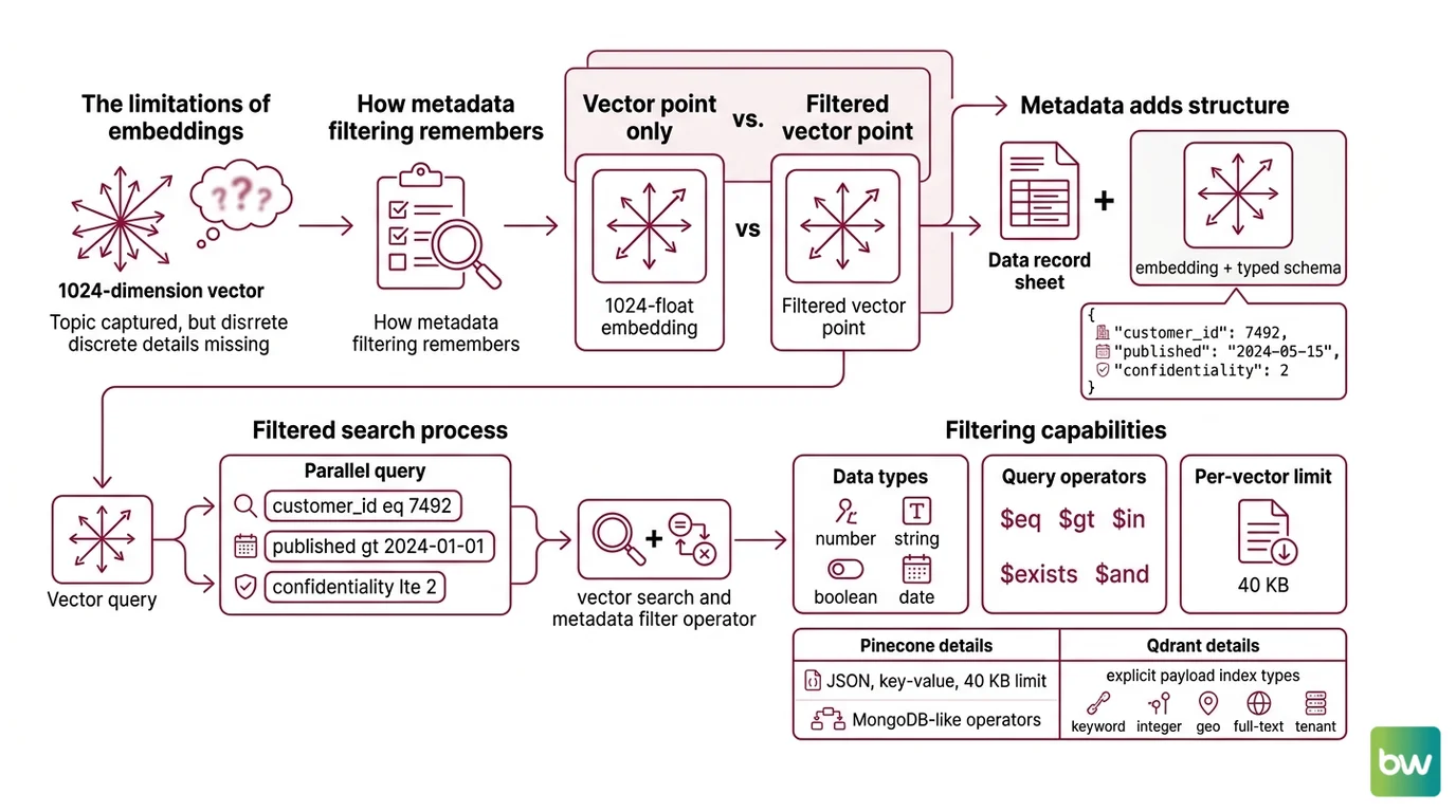
Embeddings compress meaning into a few hundred floating-point numbers. That compression is the source of their power and the source of their amnesia. A 1024-dimension vector that captures the topic of a Document Parsing And Extraction pipeline output cannot also encode that the document belongs to customer 7492, was published on a Wednesday, and is classified at confidentiality level 2. Those facts live in a different space — a typed, discrete, queryable one — and metadata filtering is what connects them back to the dense vector.
What is metadata filtering in vector search?
Metadata filtering is the practice of attaching structured key-value payload to each vector and applying predicates over those fields during search, restricting results beyond pure semantic similarity (Weaviate Docs). A vector point is no longer just a 1024-float embedding; it is an embedding plus a small JSON-like record — {"tenant_id": 7492, "language": "en", "published_at": 1735603200, "confidentiality": 2} — and queries become two-part objects: a query vector plus a boolean expression over those fields.
Pinecone exposes this as JSON key-value pairs supporting numbers, strings, booleans, and lists of strings, with a per-vector limit of 40 KB on the standard tier (Pinecone Docs). The filter language is modeled on MongoDB query operators — $eq, $ne, $gt, $gte, $lt, $lte, $in, $nin, $exists, $and, $or — with a hard cap of 10,000 values per $in or $nin clause. Qdrant takes the same idea further, supporting payload index types for keyword, integer, float, geo, full-text, tenant, on-disk, and parameterized fields, each created explicitly per field rather than implicitly inferred (Qdrant Docs).
The structural difference between an unfiltered system and a filtered one is not the embeddings. It is that the second system has a typed schema sitting beside the vector index, and a query language that lets predicates over that schema participate in retrieval.
How does metadata filtering work alongside semantic similarity in RAG systems?
This is where the problem stops being notation and starts being geometry. There are three strategies for combining a filter predicate with an approximate nearest neighbor search, and each one fails in a different way.
Pre-filtering computes the filter first, produces an allow-list of candidate IDs, then runs ANN over only those points. It guarantees that every returned vector satisfies the predicate. The trap: when the filter is selective enough to disconnect the HNSW graph, the search algorithm cannot reach the matching points through the surviving links, and recall collapses (Qdrant Blog). The graph was built assuming all nodes are reachable; the filter quietly violates that assumption.
Post-filtering does the opposite — it runs the unfiltered ANN search first, then drops any returned points that fail the predicate. The vector index stays whole. The trap: when the filter is highly selective, the top-k unfiltered results may contain few or even zero matching points, forcing the system to either return too little or run the search again with a larger k. Compute is wasted on points the user will never see.
In-algorithm filtering — the modern approach — pushes the predicate into the index traversal itself. The graph search is filter-aware: it skips non-matching points but still traverses through them, or maintains alternative paths so the graph stays connected. Qdrant’s filterable HNSW adds extra graph links between filter-matching points so the index stays connected after filtering, preserving recall (Qdrant Docs). ACORN, introduced by Patel, Kraft, Guestrin, and Zaharia in 2024, is a predicate-agnostic variant that uses two-hop neighbor expansion to maintain reachability under arbitrary filters; the paper reports throughput gains in the range of 2-10× on low-cardinality predicates and up to roughly 1,000× on 25-million-vector datasets versus prior methods, depending on selectivity and recall target (arXiv). ACORN became the default filter strategy in Weaviate v1.34, replacing the earlier “sweeping” approach (Weaviate Blog).
The mechanism is not a single algorithm but a family of trade-offs, and naming them is the first step to predicting where your retrieval will silently misbehave.
The Three Components Hidden Inside Every Filtered Vector Search
Vendors describe their filter systems in different vocabularies, but the conceptual decomposition is consistent across Qdrant, Pinecone, Weaviate, and Milvus. Three things have to be true for filtered retrieval to work, and each one is a system in its own right.
What are the components of a metadata filtering system: payload schema, filter index, and query planner?
The first component is the payload schema — a typed, per-field declaration of what each vector knows about itself beyond its embedding. Pinecone’s flat JSON model is the minimalist version: numbers, strings, booleans, lists of strings (Pinecone Docs). Qdrant’s typed payload indexes are the maximalist version: a developer must declare, per field, whether it is a keyword (exact match), integer (range queries), geo (radius queries), text (full-text search), or tenant (multi-tenant isolation) field, because the index structure differs for each (Qdrant Docs). The schema is what makes the filter language meaningful — $gte over a string is incoherent; $gte over a typed integer field has a well-defined index path. This is the same instinct that drives
Knowledge Graphs For RAG: structured retrieval needs typed facts, not just dense vectors.
The second component is the filter index — a secondary data structure that maps payload values to point IDs, sitting alongside the vector index. Qdrant’s filter index is an inverted structure where, for example, category: laptop → {1, 4, 7} (Qdrant Blog). Weaviate uses an inverted index that builds an “allow-list of eligible candidates,” and the HNSW index then only emits IDs present on that list (Weaviate Docs). Milvus scans scalar fields, marks rows to ignore, and runs ANN ignoring those rows — the same idea expressed as a bitmap (Milvus Docs). The structure varies; the function does not. Without this index, every filter degenerates into a full payload scan, and the cost of filtering grows linearly with collection size.
The third component is the query planner — the part that decides, at query time, which strategy to apply. Qdrant’s planner estimates filter cardinality and chooses between a payload-index scan with exact rescore (when the predicate is highly selective) and filterable HNSW (when the predicate is broad), because the breakeven point between those two strategies depends on what fraction of the corpus the filter admits (Qdrant Blog). Pinecone’s serverless engine integrates filters directly into the vector retrieval path over LSM-tree slabs in object storage, validated on YFCC and production data with categorical and numeric fields (Pinecone Research). The planner is where the math meets the workload.
If any of the three is missing, filtered retrieval either fails to scale or fails to be correct. Other systems implement equivalents under different names — some do not expose the planner as a separate concept — but the three responsibilities are always there, somewhere.
What This Predicts About Your Retrieval
Once the three-component model is in place, certain failure modes become predictable rather than surprising. The mechanism tells you where to look.
- If your collection grows past a few million points and filtered queries become slow, the missing piece is almost always the filter index — somebody added the payload field but never declared an index over it, so every query is doing a full scan.
- If your top-k results contain points that violate the filter, the system is using post-filtering and the unfiltered candidate pool was too small; widen k or move to a pre-filter or in-algorithm strategy.
- If your recall drops sharply when a previously-broad filter becomes selective, the HNSW graph has likely become disconnected under the filter; this is the classic failure ACORN and filterable HNSW were built to address.
- If you see correct results in development and wrong results in production, suspect the planner: small collections look fast under any strategy, and the cardinality estimator only earns its keep at scale.
Rule of thumb: Decide the predicate model before you decide the embedding model. The shape of your filters determines which database fits, and that decision is much harder to reverse than swapping a sentence-transformer.
When it breaks: Combining hybrid (lexical + vector) search with strict pre-filters is fragile across engines. Weaviate users have reported configurations where strict pre-filtering becomes unreliable when hybrid search is layered on top (Weaviate GitHub) — production systems that mix BM25 and vector ranking with metadata constraints should validate end-to-end behavior rather than trust the documented contract.
Compatibility notes:
- Weaviate filter strategy: Default changed to ACORN in v1.34. Pre-1.34 docs describe different default behavior — verify which version your cluster runs before debugging recall.
- Weaviate hybrid + filter: Open issue #7681 reports unreliable strict pre-filtering when combining hybrid search with filters. Production users should validate the behavior for their specific configuration.
- Pinecone metadata size: The 40 KB per-vector limit applies to the standard tier; serverless and other tiers may differ — verify current docs before designing payload schemas.
The Data Says
Metadata filtering is what turns a vector database from a similarity engine into a retrieval engine. The unsolved part of vector search was never “how do I find the closest point” — it was “how do I find the closest point that also satisfies the constraints my application has.” The three-component model — payload schema, filter index, query planner — describes how every modern engine answers that question, and the trade-off space among pre-filter, post-filter, and in-algorithm strategies is where most production retrieval bugs hide.
AI-assisted content, human-reviewed. Images AI-generated. Editorial Standards · Our Editors