What Is Continuous Batching and How Iteration-Level Scheduling Maximizes GPU Throughput
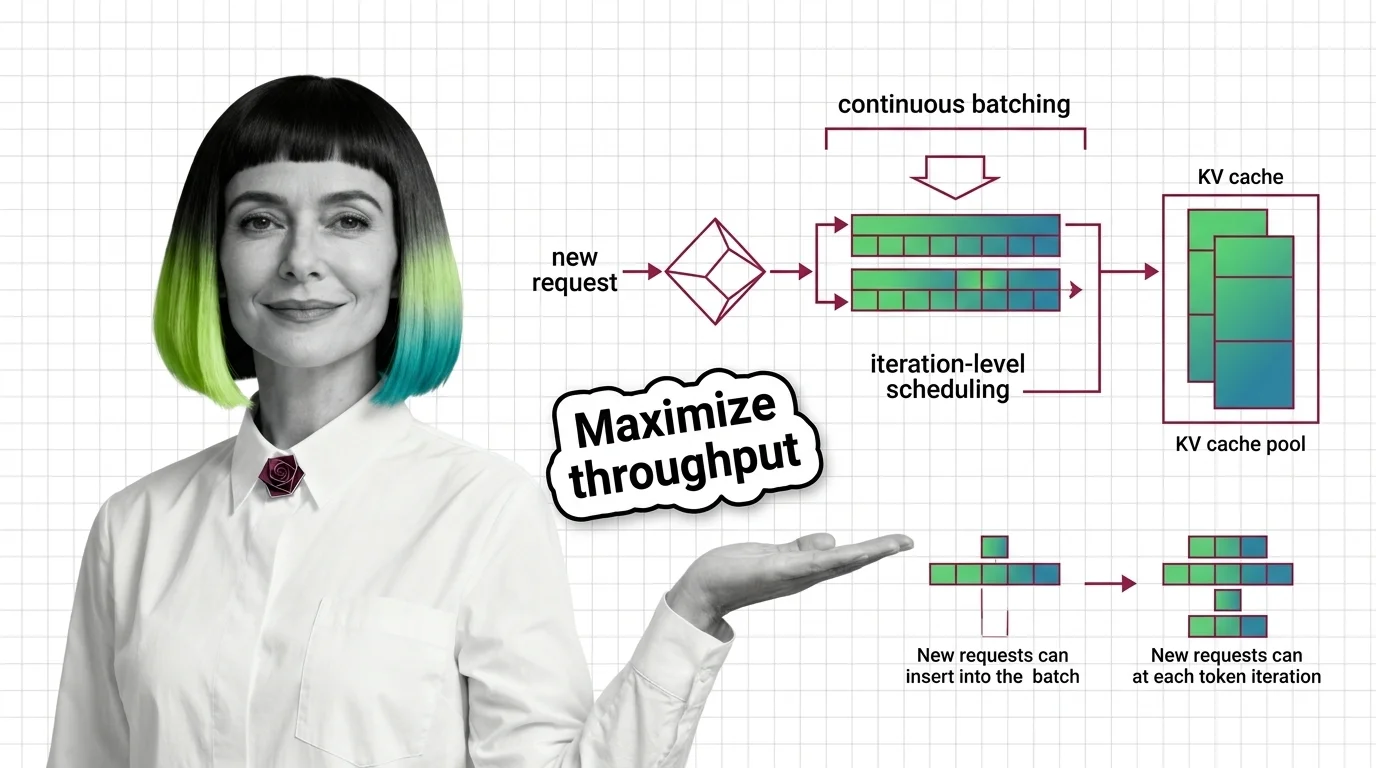
Table of Contents
ELI5
Instead of waiting for every request in a group to finish before starting new ones, continuous batching slots new requests into the GPU the instant any running request completes — keeping hardware busy on every single forward pass.
Picture a restaurant where no table can be cleared until every diner in the room finishes eating. A party of two waits forty minutes because someone across the room ordered the tasting menu. That is static batching — and until 2022, it was the default way most Inference servers handled LLM requests. The waste, once you measure it, is architectural.
Static Batching and the Geometry of Wasted Cycles
The intuition behind batching is sound: group requests together, amortize the cost of loading model weights across all of them. GPUs are parallel processors — they thrive on simultaneous work. And they do, for exactly one phase of inference: the prefill, where input tokens are processed in parallel.
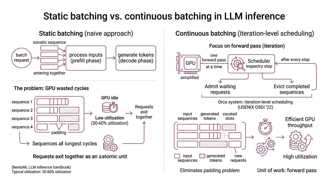
The problem arrives in the decode phase. Autoregressive generation produces tokens one at a time, sequentially. Each request in a batch generates at a different rate, finishes at a different time, and needs a different number of output tokens. Static batching — sometimes called naive batching — treats the batch as an atomic unit. Every request enters together. Every request leaves together. The GPU sits partially idle while short sequences pad their outputs with nothing, waiting for the longest sequence to complete.
The result: GPU utilization between 30% and 60% under typical static batching workloads (BentoML LLM Inference Handbook). Machines burning kilowatts of power, half the time doing arithmetic on padding tokens that carry zero information.
What is continuous batching in LLM inference?
Continuous batching is a scheduling strategy that operates at the iteration level rather than the request level. Instead of locking a batch until all sequences finish, the scheduler inspects the batch after every single forward pass — every decode step — and makes two decisions: which completed sequences to evict, and which waiting requests to admit.
The concept was introduced by Yu et al. in the Orca system (USENIX OSDI ‘22), which coined the term “iteration-level scheduling.” The insight is deceptively simple: the natural unit of GPU work in autoregressive generation is not the request. It is the forward pass.
Not the request. The iteration.
Once you shift scheduling granularity to the iteration, the padding problem dissolves. A sequence that finishes after 50 tokens releases its slot immediately, and a new request fills that slot on the very next forward pass. The GPU never waits for stragglers — and that changes the economics of every decode cycle that follows.
The Forward-Pass Clock: How Requests Enter Mid-Generation
Traditional batching opens the gate, processes everyone, closes the gate. Continuous batching turns the decode loop into something closer to a revolving door — it checks the gate on every tick of the forward-pass clock.
How does continuous batching insert new requests while other sequences are still generating tokens?
The mechanism works in three phases per iteration:
Eviction. After each forward pass, the scheduler checks which sequences have produced their end-of-sequence token or hit the maximum length. These sequences are removed from the active batch and their results are returned to the client. Their KV Cache memory is released immediately.
Admission. The scheduler then inspects the request queue. If the active batch has open slots — because sequences were just evicted — new requests are pulled from the queue. Each incoming request undergoes its prefill computation; some systems fuse this into the same forward pass (fused prefill-decode), others handle it as a separate micro-step.
Execution. The newly composed batch — a mix of requests at various stages of generation — runs the next forward pass together. A request on its second token sits alongside a request on its two-hundredth token. The GPU processes them all in parallel; it does not distinguish early-stage from late-stage sequences within the same forward pass.
This per-iteration scheduling is what drives the throughput advantage. Benchmarks show roughly an 8x improvement over static batching from the scheduling mechanism alone (Anyscale Blog). When combined with memory optimizations like PagedAttention — which manages the KV cache as virtual-memory-style pages rather than contiguous blocks — throughput improvements can climb substantially higher. But the foundation is the scheduling granularity shift; everything else builds on top of it.
Inside the Scheduling Engine
A continuous batching system is not a single algorithm. It is an architecture — a set of cooperating components that make the per-iteration scheduling loop possible. Understanding why each component exists reveals where the performance gains actually come from.
What are the key components of a continuous batching system including scheduler request queue and KV cache pool?
The request queue holds incoming requests in arrival order — or by priority, depending on the implementation. The queue is the buffer between the network layer and the scheduling loop. Its depth determines how much burst traffic the system can absorb before it must reject or throttle new connections.
The scheduler is the decision-maker. On every iteration, it reads the state of the active batch and the queue, then decides how many new requests to admit. The decision is constrained by two resources: compute (how many sequences can run in parallel without exceeding memory bandwidth) and memory (how much KV cache space remains available). In Text Generation Inference, tuning parameters such as WAITING_SERVED_RATIO and MAX_WAITING_TOKENS control the balance between latency for in-progress requests and throughput for queued ones.
The KV cache pool is the critical memory resource. Every active sequence maintains a key-value cache that grows with each generated token. In static systems, this cache is pre-allocated as contiguous blocks — wasteful when sequence lengths vary wildly. PagedAttention, introduced by Kwon et al. (SOSP ‘23), restructured the KV cache into fixed-size pages that can be allocated and freed independently, much like virtual memory pages in an operating system. This reduced internal fragmentation and enabled the scheduler to pack more sequences into GPU memory simultaneously — yielding 2-4x additional throughput at equivalent latency.
The model execution engine performs the actual forward pass. It receives the composed batch from the scheduler and runs attention, feed-forward, and sampling computations. Quantization of model weights directly affects how many sequences the engine can process in parallel, since smaller weight representations free GPU memory for more KV cache entries. The relationship is not merely additive; it interacts with the scheduler’s admission decisions at every iteration.
What the Scheduling Geometry Predicts
The shift from request-level to iteration-level scheduling changes the performance profile in predictable ways — and introduces its own failure modes.
If your workload has high variance in output length (some requests generate 20 tokens, others generate 2,000), continuous batching provides the largest gains. The more uneven the sequence lengths, the more padding cycles static batching wastes, and the more continuous batching recovers. GPU utilization can reach 80-95% under favorable conditions, though the exact figure depends heavily on sequence length distribution, model size, and batch capacity.
If you serve many concurrent users with Temperature And Sampling settings that produce variable-length outputs, the GPU stays consistently saturated. If you serve few users with predictable output lengths — a structured extraction task that always returns 50 tokens, say — the advantage narrows substantially. The scheduling geometry favors variance; uniformity gives it less room to work.
Rule of thumb: if your output lengths vary widely across requests, continuous batching is not optional — it is the difference between the 30-60% GPU utilization of static batching and the 80-95% that iteration-level scheduling can achieve.
When it breaks: continuous batching degrades when KV cache memory becomes the bottleneck rather than compute. A sudden spike of long-context requests can exhaust the cache pool, forcing the scheduler to throttle admission and effectively recreating the queuing delays it was designed to eliminate. Memory pressure, not compute, is the typical failure mode.
Compatibility notes:
- TGI maintenance mode: Hugging Face moved TGI to maintenance mode in December 2025, recommending vLLM or SGLang for new deployments (HF TGI GitHub).
- vLLM V0 engine: The legacy V0 engine in vLLM is deprecated as of v0.18.0; code removal is planned for end of June 2026 (vLLM Releases).
The Data Says
Continuous batching is not an optimization trick. It is a scheduling paradigm shift — from treating the request as the atomic unit to treating the forward pass as the atomic unit. That single change, introduced in the Orca system in 2022, turned GPU utilization from a structural waste problem into an engineering variable you can measure and control. The frameworks that implement it are converging on similar architectures; the question for most teams is no longer whether to adopt iteration-level scheduling, but which engine’s memory management best fits their workload.
AI-assisted content, human-reviewed. Images AI-generated. Editorial Standards · Our Editors