What Is an Embedding and How Neural Networks Encode Meaning into Vectors
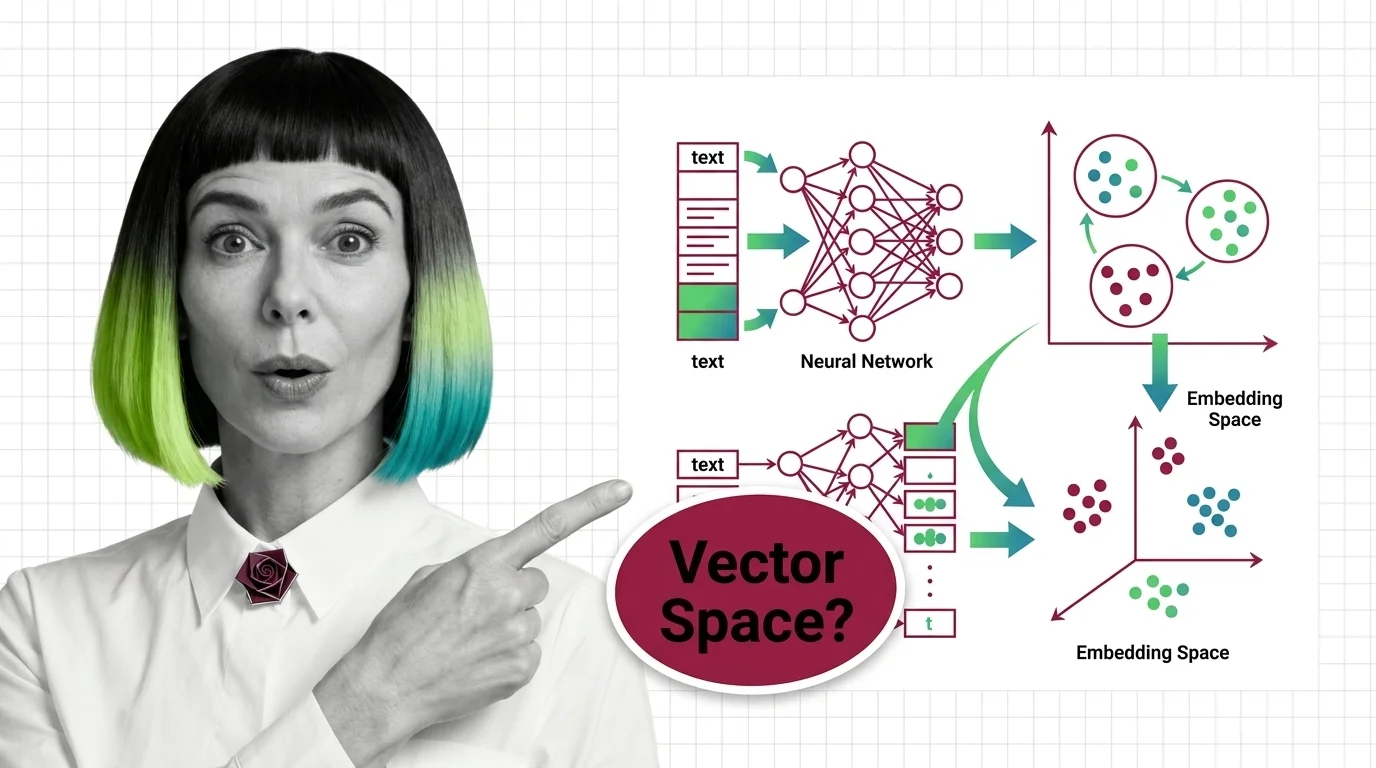
Table of Contents
ELI5
An embedding turns a word, sentence, or image into a list of numbers — a coordinate in geometric space — so that similar meanings land close together and different meanings land far apart.
Here is something that should not work. Take the vector for “king,” subtract “man,” add “woman.” The result lands nearest to “queen.” Arithmetic on words — as if meaning were something you could add and subtract like voltage in a circuit.
It is not a parlor trick. It is geometry, learned from billions of sentences, and it reveals something unsettling about how language carries structure that humans use fluently but never see directly.
The Coordinate System Hidden Inside Language
Every embedding model builds something you never asked for: a coordinate system where proximity encodes meaning. Before you touch a single API call or vector database, the underlying math is simpler — and stranger — than most explanations admit.
What is an embedding in machine learning and NLP?
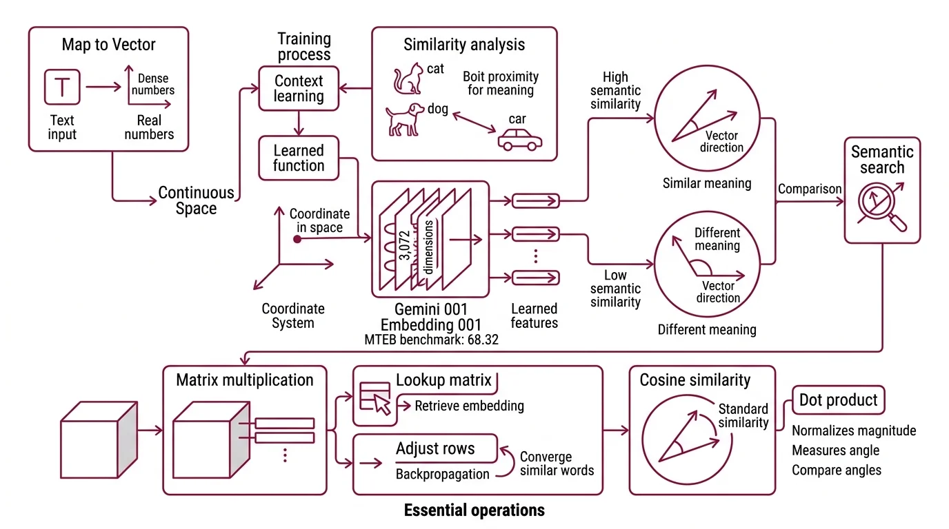
An embedding is a learned function that maps a discrete symbol — a word, a sentence, a pixel grid — to a dense vector of real numbers in continuous space. The key word is “learned.” Unlike a one-hot encoding where “cat” and “car” are equally distant from “dog,” an embedding places “cat” and “dog” nearby because the training data showed them in similar linguistic contexts.
The result is a point in high-dimensional space. Google’s Gemini Embedding 001 produces vectors with 3,072 dimensions and, as of March 2026, holds the top position on the English MTEB benchmark at 68.32 (Google Developers). Those are not arbitrary columns in a spreadsheet — each dimension encodes a learned feature, and the constellation of features defines what the model has extracted about a word’s role in language.
The practical consequence: two pieces of text with similar meaning produce vectors that point in roughly the same direction. Two pieces with different meaning point elsewhere. Semantic Search exploits this directly — instead of matching keywords character by character, you compare the angle between vectors.
Not keyword matching. Geometric nearness.
What linear algebra and neural network concepts do you need to understand embeddings?
Three operations carry most of the weight.
Matrix multiplication — the embedding layer in a neural network is a lookup matrix where each row corresponds to a token in the vocabulary. Retrieving an embedding means selecting a row. Training means adjusting every row through backpropagation so that contextually similar words converge to similar vectors.
Cosine similarity — the standard metric for comparing embeddings. It measures the cosine of the angle between two vectors; a value of 1.0 means identical direction, 0 means orthogonal, and -1 means opposite. Direction matters more than magnitude, which is why cosine similarity dominates over Euclidean distance in most retrieval systems.
Dimensionality Reduction — humans cannot visualize 3,072 dimensions. Techniques like t-SNE and UMAP project high-dimensional embeddings into 2D or 3D, revealing cluster structures — topic groups, sentiment gradients, syntactic families — that would remain invisible otherwise. The clusters are real; the 2D layout is a useful approximation.
If you understand these three, you understand the geometry. Everything else — attention heads, positional encodings, contrastive losses — is an optimization on top of this foundation.
How a Network Learns to Place Meaning in Space
The geometry does not arrive pre-built. It emerges from a deceptively simple training signal: predict what comes next, or predict what is missing, from context. The network that solves this prediction task builds — as a side effect — a representation of meaning that nobody explicitly programmed.
How do neural networks learn embedding representations during training?
The original insight came from Word2vec. Mikolov, Chen, Corrado, and Dean published two architectures in 2013: CBOW, which predicts a target word from its surrounding context, and Skip-gram, which inverts the problem — predicting context words from a single target (Mikolov et al.). Neither architecture was designed to produce meaningful geometric relationships. The vectors were a means to an end; the prediction task was the objective.
But the means turned out to be more valuable than the end.
During training, words that appear in similar contexts get pulled toward similar regions in vector space. “Paris” and “Berlin” converge — not because anyone labeled them as capitals, but because the sentences surrounding them share statistical patterns. The structure is emergent, not engineered.
GloVe took a different path. Pennington, Socher, and Manning factorized a global word co-occurrence matrix, turning raw frequency counts into dense vectors (Pennington et al.). The approach was more explicitly algebraic — matrix factorization rather than gradient descent on prediction — and yet it produced the same king-queen analogy structure that Word2Vec discovered through a completely different training objective.
Two architectures. Different training signals. Same geometric outcome.
That convergence is the strongest evidence that the geometry is not an artifact of one particular method — it is a property of language itself, waiting to be extracted.
What are the differences between word embeddings, sentence embeddings, and multimodal embeddings?
Word embeddings assign one vector per token. The limitation is immediate: “bank” gets the same coordinates whether it means a riverbank or a financial institution. Context vanishes at the token boundary.
Sentence embeddings solve this by encoding an entire input sequence into a single vector. Sentence-BERT, introduced by Reimers and Gurevych in 2019, fine-tuned BERT using Siamese and Triplet network architectures to produce sentence-level representations where semantic similarity could be computed with a single cosine comparison. This was the architectural bridge that made Dense Retrieval practical at scale — comparing full passages by geometric proximity, not individual words by string overlap.
Multimodal embeddings extend the coordinate system further. Cohere’s Embed v4 maps text, images, and PDFs into the same 1,536-dimensional space with Matryoshka Embedding support at 256, 512, 1,024, and 1,536 dimensions (Cohere Docs). A photograph and a paragraph describing its contents can occupy the same coordinates — not because they share tokens, but because they share meaning across modalities.
The progression from word to sentence to multimodal is not merely wider input. It is a shift from static vocabulary lookups to dynamic, context-sensitive, modality-agnostic representations — and each step demanded a fundamentally different training architecture to achieve.
Where the Coordinates Predict — and Where They Lie
The geometry gives you practical leverage — and practical traps. If two embeddings are close, the system treats their meaning as interchangeable for search, clustering, and recommendation. The if/then predictions follow directly from the math.
If you reduce embedding dimensions using Matryoshka techniques, you trade precision for speed. Kusupati et al. demonstrated that nested embeddings retain roughly 98% of retrieval performance at 8% of the original vector size (Kusupati et al.). For latency-sensitive applications — autocomplete, real-time filtering — this trade-off makes the architecture viable without rebuilding the index.
If you compare MTEB benchmark scores across models, read the task-level breakdown, not the headline average. Overall averages mislead; a model can score high on classification while underperforming on retrieval (MTEB). Cross-leaderboard comparisons between English and multilingual benchmarks deserve even more caution — different evaluation sets measure different capabilities.
If you switch embedding models mid-project, every stored vector becomes incompatible. Embeddings from different models occupy different coordinate systems. There is no universal translation layer between them; you re-embed your entire corpus or you accept silent inconsistency in your results.
Rule of thumb: Choose your embedding model before you build your index, and treat that choice as infrastructure — not a parameter you swap on a Tuesday afternoon.
When it breaks: Embeddings fail silently on out-of-distribution input. A model trained predominantly on English text will still return a vector for Mandarin input — the cosine similarity will look numerically normal, the coordinates will occupy real space, but the meaning will be noise. The geometry works only within the distribution the model has actually seen. There is no error message. Just confident nonsense.
Compatibility notes:
- Gensim (Word2Vec/GloVe):
glove2word2vecis deprecated. UseKeyedVectors.load_word2vec_format(binary=False, no_header=True)instead.- Sentence Transformers v5.3.0 (March 2026): Requires Transformers v5.0+. Models saved with v2.x may fail on v5.x.
The Data Says
Embeddings are not a feature. They are the representation layer that determines whether a system can distinguish meaning from syntax. The mechanism is linear algebra; the training signal is context prediction; the failure mode is silent — vectors always exist, even when they encode nothing useful. Every retrieval system, every recommendation engine, every clustering pipeline inherits the quality and the blind spots of the embedding model underneath it.
AI-assisted content, human-reviewed. Images AI-generated. Editorial Standards · Our Editors