What Is a Variational Autoencoder and How the Reparameterization Trick Enables Generative Learning
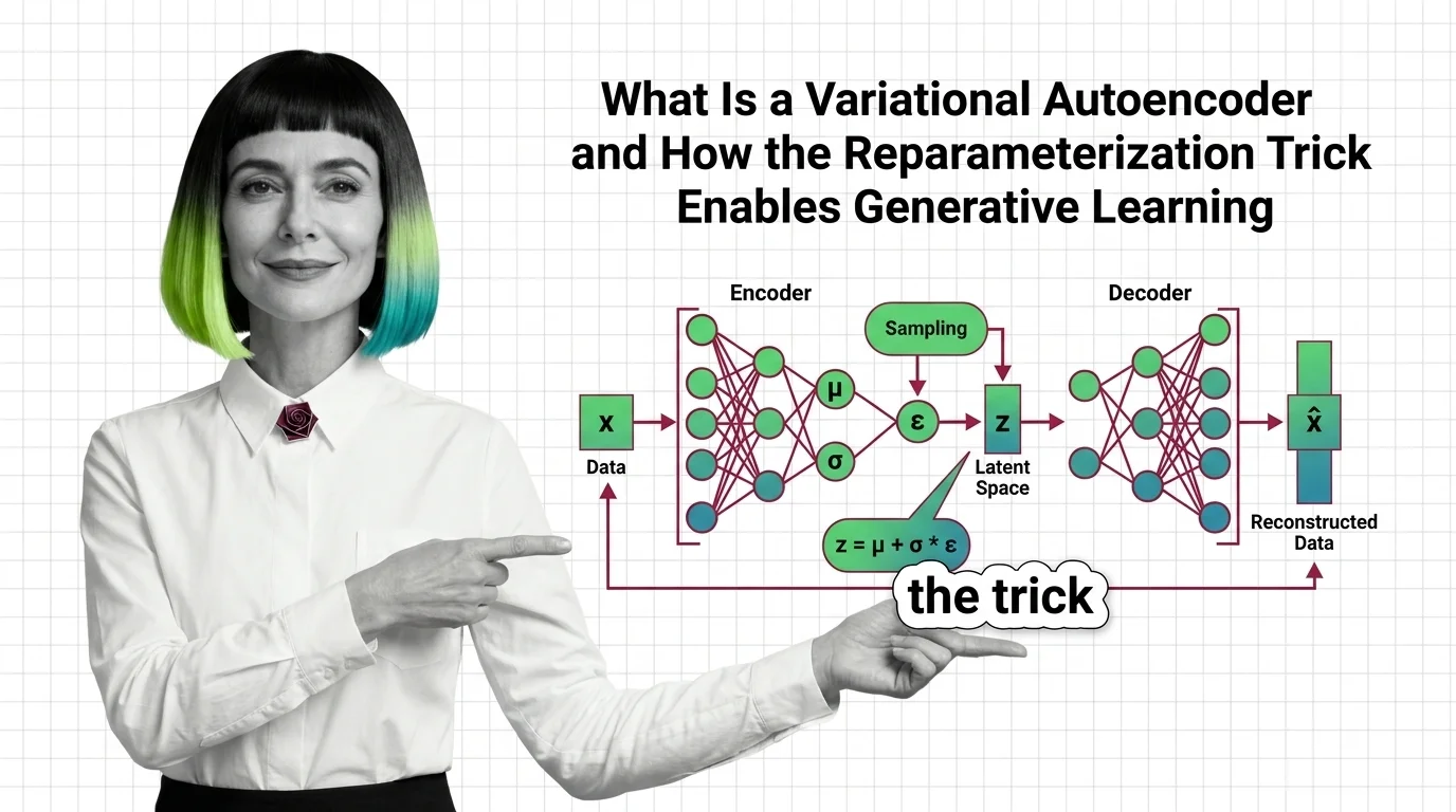
Table of Contents
ELI5
A variational autoencoder compresses data into a smooth probability space, then generates new samples by decoding points from that space. The reparameterization trick makes this sampling step differentiable — so the network learns end-to-end through backpropagation.
Here is something that should bother you about generative models: they require randomness at their core — sampling from a probability distribution — yet Backpropagation demands a deterministic, differentiable path from output back to input. These two requirements are, on paper, incompatible. The variational autoencoder resolves this contradiction with a piece of algebra so simple it almost feels like cheating. Almost.
The Compression Machine That Thinks in Probability
Most autoencoders learn to compress. They push data through a bottleneck and reconstruct it on the other side — a forced lossy copy. The variational autoencoder does something structurally different. It doesn’t compress data into points; it compresses data into distributions. That single change — from coordinates to probability clouds — is what separates a compression tool from a generative model.
What is a variational autoencoder
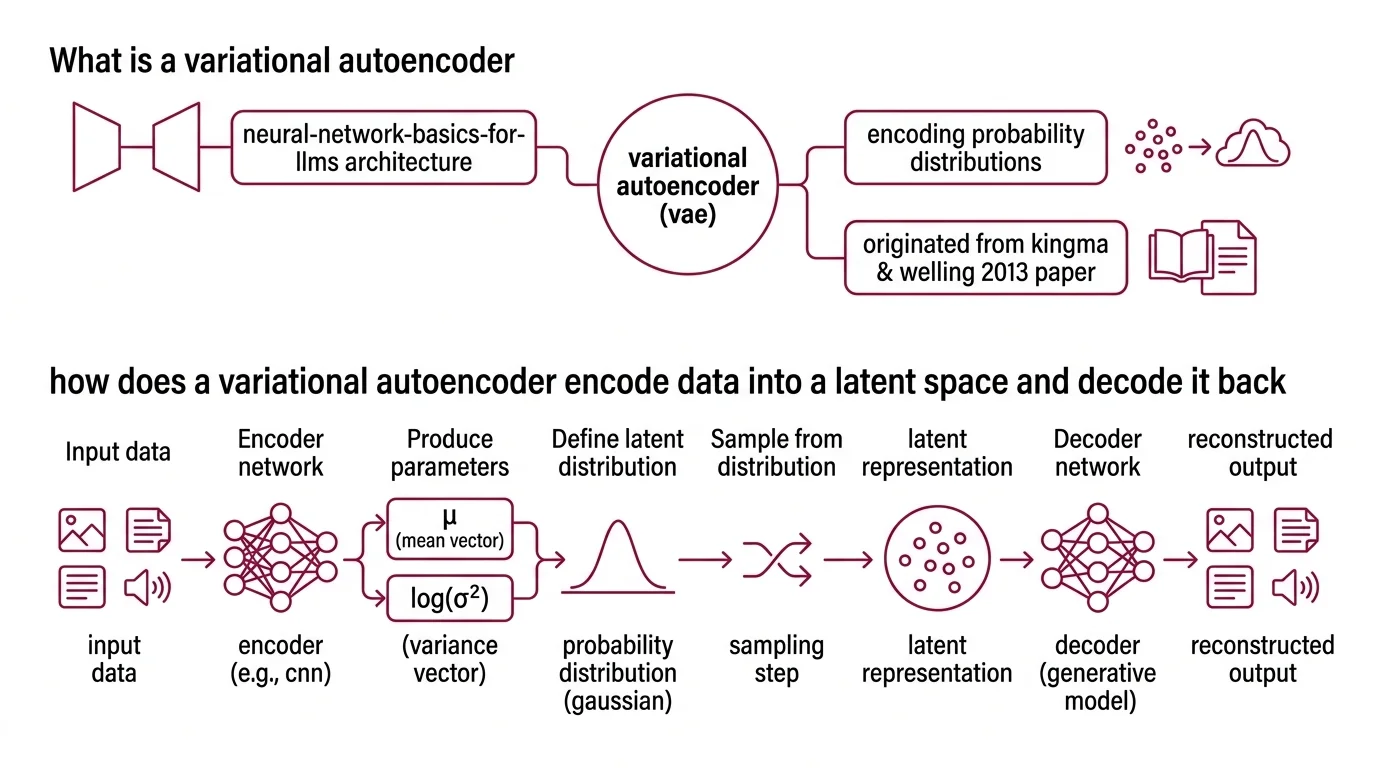
A variational autoencoder is a Neural Network Basics for LLMs architecture with two halves: an encoder that maps input data to a probability distribution in a lower-dimensional latent space, and a decoder that maps samples from that space back to data. The encoder doesn’t output a single compressed representation — it outputs the parameters of a distribution, specifically a mean vector (μ) and a variance vector (σ²), defining a Gaussian cloud for each input.
The original framework was introduced by Kingma and Welling in their 2013 paper “Auto-Encoding Variational Bayes” (Kingma & Welling, 2013), published at ICLR 2014. What made the paper significant was not the encoder-decoder structure — autoencoders had existed for decades — but the probabilistic formulation that turned compression into inference.
The decoder, in this framework, is a generative model. Give it any point in the latent space, and it will attempt to produce a plausible data sample. Whether it succeeds depends entirely on how well-organized that latent space has become during training — which depends, in turn, on a loss function with two competing terms and a gradient trick that shouldn’t work but does.
How does a variational autoencoder encode data into a latent space and decode it back
The encoding step works like this: a Convolutional Neural Network (or any architecture suited to the data type) processes the input and produces two vectors — μ and log(σ²). These define a Gaussian distribution in the latent space. The input image of a face, for instance, doesn’t map to a single point; it maps to a region of possibility.
The decoder receives a sample z drawn from that region and reconstructs the original data. In practice, decoder architectures mirror the encoder — if the encoder uses convolutional layers, the decoder uses transposed convolutions. The output is not a perfect copy; it is the decoder’s best probabilistic guess given the sampled latent code.
This is where the architecture diverges from a standard autoencoder. A standard autoencoder encodes to a fixed point and decodes from that same point — deterministic, brittle, and with no guarantee that the space between encoded points means anything useful. A VAE encodes to a distribution and decodes from a sample — stochastic, smooth, and navigable.
The consequence is geometric. Move smoothly between two latent codes in a trained VAE, and the decoded outputs change smoothly too. Interpolate between the encoding of a “3” and a “7,” and you get plausible intermediate digits — not noise, not artifacts, but a gradual morphing that respects the structure of the data. That continuity property is exactly what generation requires. But training a network to produce these distributions requires gradients to flow through sampling — and that turns out to be the hard part.
The Gradient Barrier — and How VAEs Break Through It
Training any neural network requires computing gradients and propagating them backward through every operation. Each step in the forward pass must be differentiable with respect to the learnable parameters. Sampling from a distribution — drawing z from N(μ, σ²) — is not differentiable. You cannot compute the gradient of a random draw with respect to the distribution’s parameters.
This is the gradient barrier. The encoder outputs μ and σ, the decoder needs z, and between them sits a stochastic operation that blocks gradient flow entirely.
What is the reparameterization trick in VAE and why is it needed for backpropagation
The reparameterization trick resolves this by rewriting the sampling operation as a deterministic function of the parameters plus an independent noise term:
z = μ + σ · ε, where ε ~ N(0, 1)
The noise ε is sampled from a fixed standard normal distribution — it carries no learnable parameters and requires no gradients. The parameters μ and σ remain fully differentiable, and backpropagation flows through the multiplication and addition without obstruction.
This technique — also known as the pathwise derivative estimator — predates deep learning by decades; it originated in operations research in the 1980s. Kingma and Welling’s contribution was recognizing that it could bridge variational inference and neural network training in a single architecture.
The effect is profound but the algebra is almost disappointingly simple. Before the trick: the model sampled z from a parameterized distribution, and gradients died at the sampling step. After: the model computes z as a deterministic transform of learnable parameters and fixed noise, and gradients flow cleanly through the entire network.
Not magic. Algebra.
The trick also reveals something about how the encoder learns. Because gradients now propagate through μ and σ, the encoder receives direct feedback about whether its chosen mean and variance produce latent codes that help the decoder reconstruct well. The encoder doesn’t just compress; it learns to compress into regions of the space where the decoder is most effective. But knowing how to flow gradients is only half the training story — the model also needs an objective function that shapes the geometry of the space itself.
Two Forces Pulling in Opposite Directions
A VAE’s Loss Function is not a single objective — it is a tension between two competing demands. This tension is the architectural engine that gives the latent space its useful properties, and understanding it explains both why VAEs work and where they fail.
VAE loss function explained how reconstruction loss and KL divergence work together
The total loss is the negative Evidence Lower Bound (ELBO), which decomposes into two terms:
Reconstruction loss measures how well the decoder recovers the original data from the sampled latent code. For images, this is typically pixel-wise mean squared error or binary cross-entropy. It answers one question: did the decoder get the data back?
KL Divergence penalty measures how far the encoder’s learned distribution q(z|x) deviates from the prior distribution p(z) — usually a standard normal N(0, 1). It answers a different question: is the latent space organized?
The ELBO itself relates to the true data likelihood through a clean identity: log p(x) = ELBO + KL(q(z|x) || p(z|x)). The gap between the ELBO and the true log-likelihood is exactly the KL divergence between the approximate and true posteriors. Maximizing the ELBO simultaneously improves the approximation and pushes up the data likelihood.
Reconstruction loss, acting alone, would produce an autoencoder with a chaotic latent space — each input mapped to a tight, isolated spike, with no meaningful structure between them. The KL penalty, acting alone, would collapse everything to the prior — a perfectly smooth space that encodes nothing at all.
The useful latent space emerges from the tension between specificity and smoothness. The reconstruction term demands that each input be distinguishable; the KL term demands that the overall distribution stay close to a navigable Gaussian. The balance point produces a latent space that is both informative — each region decodes to a distinct data type — and continuous — nearby regions decode to similar outputs.
This is the mathematical reason VAEs generate blurrier images compared to GANs. The KL penalty actively discourages the kind of sharp, narrow distributions that would produce crisp outputs. The blurriness is not a defect in the implementation. It is the cost of a well-organized latent space.
What the Latent Geometry Predicts — and Where It Fails
The practical consequences of this architecture are geometric.
If you train a VAE on faces and interpolate between two latent vectors, the decoded outputs will transition smoothly — gradually shifting expression, pose, lighting. This works because the KL penalty forces the encoder to spread its representations across a continuous, roughly Gaussian region. No dead zones, no discontinuities.
If you increase the weight of the KL term relative to reconstruction loss, you get a smoother latent space at the cost of blurrier outputs. If you decrease it, you get sharper reconstructions but a fragmented space that fails at generation. The balance is application-specific and rarely optimal at default settings.
The architecture has become a foundational component in systems far beyond simple image generation. In Latent Diffusion models like Stable Diffusion, a pretrained VAE compresses high-resolution images into a compact latent space where the diffusion process operates — running diffusion in pixel space would be computationally prohibitive. The SD3 architecture uses a VAE with 16 latent channels, achieving roughly 12× compression compared to the 4 channels and 48× compression in SDXL (Stability AI; Ollin Boer Bohan). Discrete variants like VQ-VAE replace the continuous Gaussian with learned codebooks of discrete tokens (van den Oord et al., 2017), trading smooth interpolation for sharper reconstructions and compatibility with autoregressive decoders.
Rule of thumb: If your downstream task needs smooth interpolation and data augmentation, a standard VAE with continuous latent space is the appropriate starting point. If it needs crisp discrete tokens for sequence modeling, look at VQ-VAE or its successors.
When it breaks: The KL penalty can overwhelm weak decoders — a failure mode called posterior collapse, where the encoder learns to ignore the input and output the prior for every data point. The latent space becomes perfectly smooth but completely empty of information. Training schedules that gradually increase the KL weight (KL annealing) are the standard mitigation, but posterior collapse remains an active research problem, particularly in Recurrent Neural Network-based sequence VAEs where the decoder is powerful enough to ignore the latent code entirely.
The Data Says
The variational autoencoder is not primarily a generative model — it is a framework for learning structured, navigable latent spaces under probabilistic constraints. The reparameterization trick is the hinge: a rewrite of sampling as deterministic computation that lets gradients flow through stochasticity. Every system that trains through a sampling bottleneck — from latent diffusion pipelines to discrete-token architectures — inherits this same trick, and the same tension between reconstruction fidelity and distributional smoothness.
AI-assisted content, human-reviewed. Images AI-generated. Editorial Standards · Our Editors