What Is a Recurrent Neural Network and How Hidden States Process Sequential Data
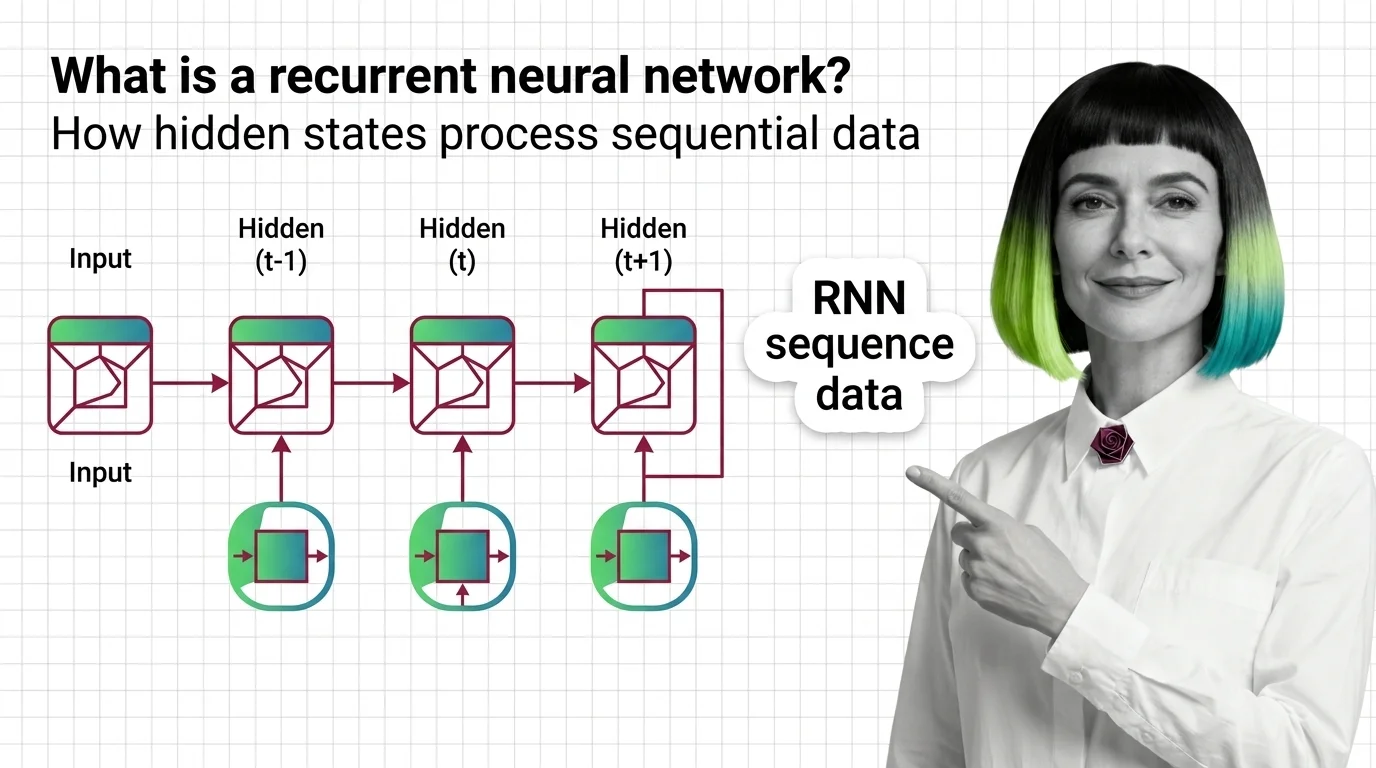
Table of Contents
ELI5
A recurrent neural network feeds its own output back as input at each time step, creating a memory loop that lets it process sequences — words, audio, time series — one element at a time while remembering what came before.
Shuffle the words in a sentence. Hand the result to a feedforward neural network, and it produces the same internal activation — completely indifferent to the reordering. Now hand it to a recurrent neural network. The output changes. Something inside the architecture is sensitive to the order in which tokens arrive, and that sensitivity comes at a cost most introductions neglect to mention.
The Loop That Gives Networks a Sense of Sequence
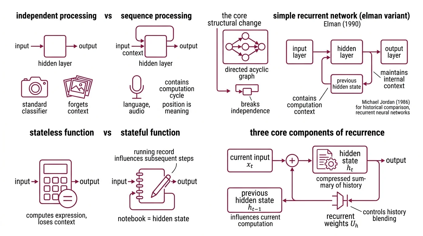
Standard Neural Network Basics for LLMs process each input independently. An image classifier examines one photograph, assigns a label, and forgets. That works for data where order carries no information — but language, audio, and stock tickers are not photographs. In these domains, position is meaning. The recurrent neural network was designed to break the independence assumption by introducing a single structural change: a feedback connection.
What is a recurrent neural network?
A recurrent neural network is a class of neural architectures where the output of a hidden layer at one time step feeds back into the same layer at the next step. Jeffrey Elman formalized this structure in 1990 as a “simple recurrent network” that learned temporal patterns by maintaining an internal context vector (Elman, 1990). Michael Jordan had proposed a related architecture in 1986 using output-to-context feedback, but Elman’s variant — feeding the hidden state itself back — became the canonical design.
The key structural difference from a feedforward network: the presence of a cycle in the computation graph. Where a feedforward network is a directed acyclic graph, an RNN has at least one edge that points backward in time. That single loop is what converts a stateless function into one with memory.
Think of it as the difference between a calculator and a notebook. The calculator computes one expression, displays the result, and loses all context. The notebook — the hidden state — keeps a running record that influences every subsequent computation.
What are hidden states, weights, and recurrent connections in an RNN?
Three components define the recurrence. The hidden state h_t is a vector that encodes a compressed summary of everything the network has observed up to time step t. The recurrent weight matrix U_h controls how much of the previous hidden state h_{t-1} bleeds into the current one. And the input weight matrix W_h determines how the new input x_t enters the computation.
The update rule is compact:
h_t = sigma(W_h * x_t + U_h * h_{t-1} + b_h)
where sigma is typically a tanh or sigmoid nonlinearity and b_h is a bias term. The output at each step depends on h_t, which in turn depends on h_{t-1}, which depends on h_{t-2}, and so on — a recursive chain that, in principle, connects the current output to the very first input.
In principle. What happens in practice is considerably less tidy, and the gap between those two words — principle and practice — is where the most interesting engineering problems live.
Following a Sentence Through the Recurrence
Definitions describe the architecture; watching the mechanism operate reveals what the architecture actually does with information over time.
How does a recurrent neural network process sequences step by step?
Consider an RNN processing the sentence “The cat sat on the mat” — six tokens, six time steps.
At t = 1, the hidden state h_0 is typically initialized to zeros. The network receives the embedding for “The” and computes h_1 using the equation above. At this point, h_1 encodes nothing interesting — just one article.
At t = 2, the network receives “cat.” Now h_2 is a function of both the embedding for “cat” and the hidden state h_1, which already contains information about “The.” The hidden state is no longer a representation of the current token; it is a compressed representation of the sequence so far.
By t = 6, when “mat” arrives, h_6 carries traces of all five preceding tokens — in theory. In practice, the contribution of earlier tokens decays with each multiplication by the recurrent weight matrix U_h. If the eigenvalues of U_h are less than one, earlier signals shrink exponentially. If they are greater than one, earlier signals explode.
Not a bug. A mathematical property of repeated matrix multiplication.
It imposes a hard limit on how far back the network can effectively look. The hidden state is a lossy compression — each step overwrites part of the previous information to make room for the new input. A Convolutional Neural Network handles spatial locality through fixed-size filters; an RNN handles temporal locality through this running compression. Both architectures make structural bets about what information to preserve.
What Exponential Decay Reveals About Learning Sequences
Training an RNN means adjusting weights so that the network produces useful outputs at each time step. The standard algorithm is backpropagation through time — BPTT — introduced by Werbos in 1990 (Werbos, 1990). BPTT unrolls the recurrence across all time steps and computes gradients as if the unrolled network were a very deep feedforward network.
The problem is mathematical, not algorithmic. Gradients flow backward through the same weight matrices that process the forward pass. When those matrices are applied repeatedly — once per time step — the gradient either vanishes or explodes exponentially. Hochreiter’s 1991 diploma thesis proved this formally: error signals decay at a rate exponential in the number of time steps, making it nearly impossible to learn dependencies spanning more than a few dozen steps.
Truncated BPTT offers a pragmatic workaround: instead of computing gradients across the entire sequence, truncate after a fixed number of steps. This introduces a slight regularizing effect but sacrifices long-range learning by design.
The real answer came in 1997. Hochreiter and Schmidhuber published Long Short-Term Memory — a gated architecture that replaces the vanilla hidden state with a cell state protected by multiplicative gates (Hochreiter & Schmidhuber, 1997). The forget gate, input gate, and output gate control what information enters, persists in, and exits the cell. The critical innovation was the constant error carousel: a path through the cell where gradients can flow without multiplicative decay, bridging time lags exceeding a thousand steps.
The Gated Recurrent Unit, proposed by Cho et al. in 2014, simplified the LSTM design by merging the forget and input gates into a single update gate and eliminating the separate output gate. Fewer parameters, faster training — at the cost of a slightly less flexible memory mechanism.
If your sequence has dependencies spanning fewer than a hundred tokens, a vanilla RNN might learn them — slowly, unreliably, but sometimes. If your dependencies span thousands of tokens, you need gating. If the relevant signal sits at position twelve in a sequence of ten thousand, even an LSTM will struggle — because the cell state, however well-gated, still compresses through a finite-dimensional bottleneck.
Rule of thumb: match the architecture to the dependency range. Short-range patterns tolerate vanilla RNNs. Long-range dependencies require gating. Ultra-long contexts are where newer architectures start to matter.
When it breaks: RNNs process sequences strictly left-to-right, one step at a time. This sequential bottleneck means they cannot be parallelized across time steps during training — a limitation that makes them orders of magnitude slower than architectures like Transformers on modern GPU hardware, and the primary reason recurrent models fell out of favor for large-scale language modeling.
Recurrence After the Transformer
For several years, the dominant narrative was simple: attention replaced recurrence. Transformers process all tokens simultaneously through self-attention, avoiding the sequential bottleneck entirely — at the cost of quadratic memory scaling with sequence length.
That trade-off is reopening the conversation. xLSTM, introduced by Beck, Hochreiter, and colleagues in 2024 and extended to a 7B-parameter language model in March 2025, reports inference speeds up to 32x faster than Transformers at 32,000-token contexts (Beck et al., 2025). The architecture introduces matrix-valued memory cells that are parallelizable during training — directly addressing the old sequential bottleneck. These claims come from the authors’ own evaluation; independent replication has not yet been confirmed as of April 2026.
Mamba, a selective state-space model from Gu and Dao published in late 2023, achieves linear-time sequence modeling with throughput roughly 5x higher than comparable Transformers, and a 3B-parameter Mamba model matched Transformer performance at twice the parameter count (Gu & Dao, 2023).
The pattern is not that recurrence has returned triumphant. The pattern is that the quadratic cost of attention at long contexts has made recurrent computation — redesigned, gated, and in some cases parallelized — competitive again in a regime where it once seemed obsolete. As of April 2026, Transformers remain dominant in production language models, but the architectural conversation is no longer a monologue.
The Data Says
Recurrence gives neural networks memory by feeding hidden states forward through time — but that memory decays exponentially unless gating mechanisms protect it. The vanishing gradient problem is not a flaw in training algorithms; it is a property of repeated matrix multiplication. Every architecture designed for sequences makes a choice about how to manage that decay, and the most consequential recent work has focused on making recurrence parallelizable without surrendering its memory advantage.
AI-assisted content, human-reviewed. Images AI-generated. Editorial Standards · Our Editors