What Is a Graph Neural Network and How Message Passing Propagates Information Across Nodes
ELI5
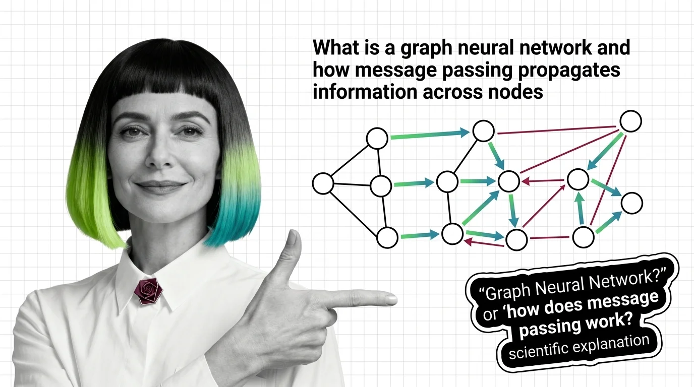
A graph neural network learns by passing messages between connected nodes — each node updates its representation based on what its neighbors encode, repeating until the whole graph captures structural patterns.
A molecule does not care about your pixel grid. Neither does a social network, a logistics route, or a protein folding pathway. These systems have structure — but not the kind that fits neatly into rows and columns. The question that graph neural networks answer is deceptively simple: what happens when you let a neural network operate on connections instead of coordinates?
The Geometry of Relationships
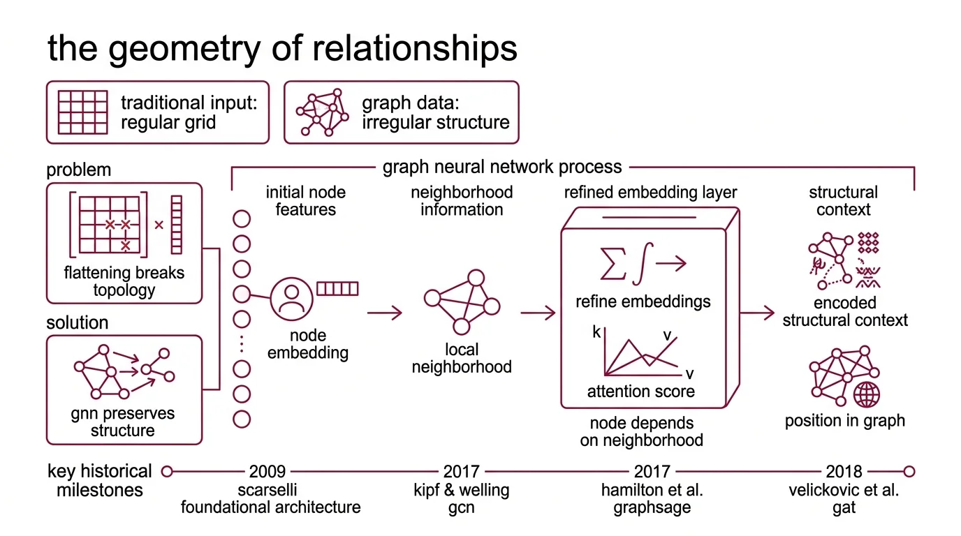
Traditional Neural Network Basics for LLMs assume input arrives on a regular grid — images as 2D pixel arrays, text as 1D token sequences. That assumption works spectacularly well when the data cooperates. The trouble begins when it doesn’t.
Consider a Knowledge Graph with ten thousand entities connected by irregular, typed relationships. Flatten it into a matrix and you destroy the very information that makes it useful — which entity links to which, and why. Graph neural networks preserve that topology by operating directly on the graph’s structure: nodes, edges, and the signals flowing between them.
What is a graph neural network?
A graph neural network is a class of neural networks designed to operate on graph-structured data — data represented as nodes connected by edges, formalized through an Adjacency Matrix. The foundational architecture was proposed by Scarselli et al. in 2009, but the field’s acceleration began when three papers arrived in rapid succession: Kipf and Welling’s Graph Convolutional Network (ICLR 2017), Hamilton et al.’s Graphsage (NeurIPS 2017), and Velickovic et al.’s Graph Attention Network (ICLR 2018).
The core insight across all three: a node’s representation should depend on its neighborhood, not just its own features. Each node starts with an initial feature vector — its Node Embedding. Through successive layers, nodes refine these embeddings by incorporating information from neighbors. After enough rounds of refinement, each node’s representation encodes not just local properties but structural context: its position in the graph, the patterns in its neighborhood, the motifs it participates in.
This is different from a standard feedforward network in a fundamental way. A feedforward layer processes a fixed-length input vector with no notion of adjacency. A GNN layer processes a variable-size neighborhood, and its output depends on the graph’s connectivity — the shape of the input changes with every node.
How does message passing work in graph neural networks?
Gilmer et al. unified the proliferating GNN architectures under a single abstraction in 2017: the Message Passing Neural Network framework (ICML 2017). The elegance lies in its simplicity — two phases, repeated across layers.
In the message phase, every node collects information from its neighbors. Each neighbor constructs a “message” — typically a function of the neighbor’s current embedding, the edge features between them, and sometimes the receiving node’s own state. These messages are aggregated, usually by summation, averaging, or a learned attention mechanism.
In the update phase, the node combines the aggregated message with its own current embedding to produce a new representation. This is the moment where neighborhood information fuses with self-information.
Stack these two phases in sequence, and you get a single GNN layer. Stack multiple layers, and information propagates further — a 2-layer GNN means every node absorbs its 2-hop neighborhood; a 3-layer GNN extends that to 3 hops. The reach of information flow equals the number of message-passing rounds.
Think of it as a telephone network where every person calls their direct contacts, summarizes what they learned, and passes the summary forward. After three rounds of calls, you know something about people three connections away — but filtered through the summaries of everyone in between. The fidelity degrades with each hop. That degradation is not a bug; it is a design constraint.
The mathematical formulation is clean: for node v at layer k, the message from neighbor u is m_uv = M_k(h_u, h_v, e_uv), where M_k is a learned message function and e_uv encodes edge features. The aggregated message is M_v = Agg({m_uv : u in N(v)}). The updated embedding is h_v’ = U_k(h_v, M_v), where U_k is a learned update function.
Different GNN variants are different choices within this framework. GraphSAGE samples a fixed-size neighborhood and concatenates the aggregation with the node’s own embedding. Graph Attention Networks assign learned attention weights to each neighbor — letting the model decide which connections matter more, rather than treating all edges as equal.
Not pixel-level patterns. Structural patterns.
Convolution Without a Grid
The word “convolution” in graph neural networks causes a specific kind of confusion — the assumption that it works the same way as in CNNs. It does not, and understanding why requires looking at what convolution actually means in both contexts.
What is the difference between graph convolution and standard convolution in neural networks?
Standard convolution in a CNN slides a fixed-size kernel across a regular grid. The kernel has a defined shape — 3x3, 5x5 — and the spatial relationships between pixels are uniform and predictable. Every pixel has the same number of neighbors at the same relative positions. This regularity is what makes the operation efficient and parallelizable.
Graphs have no such regularity. Node A might have two neighbors; node B might have two thousand. The “positions” of neighbors are defined by connectivity, not coordinates. There is no fixed kernel shape that applies here, because the neighborhood itself has a different topology for every node.
Graph convolution solves this by replacing spatial locality with topological locality. Instead of “the pixels within a 3x3 window,” the neighborhood becomes “every node connected by an edge.”
Two approaches emerged. The spectral approach — rooted in Spectral Graph Theory — defines convolution through the graph’s eigendecomposition. Kipf and Welling showed that a first-order Chebyshev approximation of spectral filters reduces to a remarkably simple operation: multiply the normalized adjacency matrix by the feature matrix and a learnable weight matrix. The full eigendecomposition disappears; what remains is a weighted average of neighbor features that can be computed efficiently.
The spatial approach skips the spectral interpretation entirely and defines convolution as direct aggregation from neighbors — exactly the message-passing framework described above. Spatial methods are generally more scalable because they avoid the eigendecomposition that spectral methods theoretically require, even when Kipf’s approximation sidesteps it in practice (a distinction well-illustrated in Distill’s visual explainer of these approaches).
The practical consequence: graph convolution is more expressive than standard convolution on irregular data, but less efficient on regular grids. If your data is an image, use a CNN. If your data is a molecule, a recommendation graph, or a fraud detection network — the grid-based kernel cannot even represent the relationships you need.
What the Topology Predicts — and Where It Stalls
The message-passing mechanism makes testable predictions. If information propagates through neighborhood aggregation, then the reach of a node’s receptive field scales linearly with the number of layers. A 3-layer GNN absorbs 3-hop neighborhoods; a 10-layer GNN should extend that to 10 hops, encoding increasingly global patterns.
If you need to capture long-range dependencies across the graph — detecting that two distant nodes in a social network share an unlikely structural pattern — you need more layers.
If you change the aggregation function from sum to attention-weighted mean, you should observe improved performance on graphs where neighbor importance varies significantly — heterogeneous networks, citation graphs, molecular systems with varied bond types.
If you add edge features to the message function, you should expect richer representations on graphs where edges carry meaningful information — molecular bonds with type and order, financial transactions with amounts and timestamps.
Rule of thumb: Match the number of message-passing layers to the diameter of the patterns you need to detect — but prepare for diminishing returns past five or six layers.
When it breaks: Oversmoothing is the central failure mode. As you stack more GNN layers, node embeddings converge — they become increasingly similar, losing the local distinctions that make them useful. A deep GNN often performs worse than a shallow one because every node’s embedding drifts toward the same global average. The research community has proposed multiple mitigation strategies — residual connections, normalization techniques, various convergence metrics — but as of 2026, the metrics themselves lack consensus; rank-based and energy-based approaches yield different conclusions about when oversmoothing actually occurs (Jin & Zhu). The problem is well-characterized. The solution remains an active research front.
The framework implementations reflect this evolving state. Pytorch Geometric (version 2.7.0, released October 2025) is the dominant library, with PyTorch-native integration and an ongoing transition from SparseTensor to a new EdgeIndex representation (PyG Docs). Deep Graph Library (version 2.4.0, released September 2024) offers multi-backend support but has shown a notably slower release cadence — some downstream projects have begun migrating to PyG.
Compatibility notes:
- PyTorch Geometric SparseTensor deprecation:
torch-sparse-based SparseTensor is being replaced by EdgeIndex/Index in PyG 2.7+. Existing code using SparseTensor should plan migration.- DGL release cadence: Last release September 2024. Not archived, but reduced activity and ecosystem migration suggest evaluating maintenance status before adopting for new projects.
The Data Says
Graph neural networks formalize a principle that grids cannot express — let structure inform representation — through a mechanism elegant enough to describe in two phases: collect messages from neighbors, update yourself. The power and the limitation live in the same place: information propagates through topology, which means the network is only as good as the graph it operates on, and only as deep as oversmoothing permits.
AI-assisted content, human-reviewed. Images AI-generated. Editorial Standards · Our Editors