What Is a Diffusion Model? How Reversing Noise Creates Images and Video

There is something cosmically strange about diffusion models. You hand them a canvas of pure random noise and they return a photograph of a dog that does not exist. No retrieval, no library — just noise, shaped into a picture. And yet FLUX.2, Stable Diffusion 3, and Veo 3 — the entire frontier of image and video generation in 2026 — is built on this operation. So what is actually happening?

What a diffusion model learns when you train it on destruction

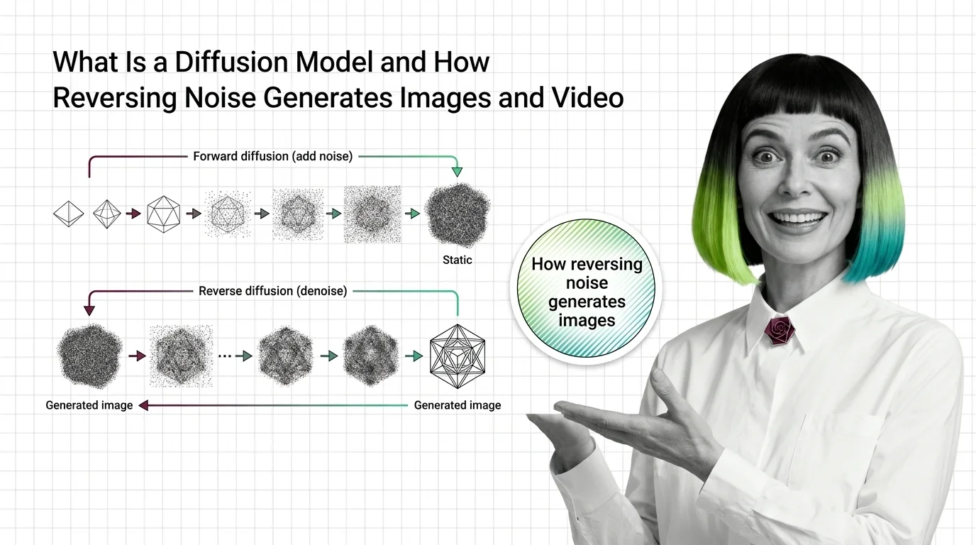
Before the reverse process there is a forward process, and the forward process is the key to the whole trick. The training target is noise, not the image.

What is a diffusion model in AI?

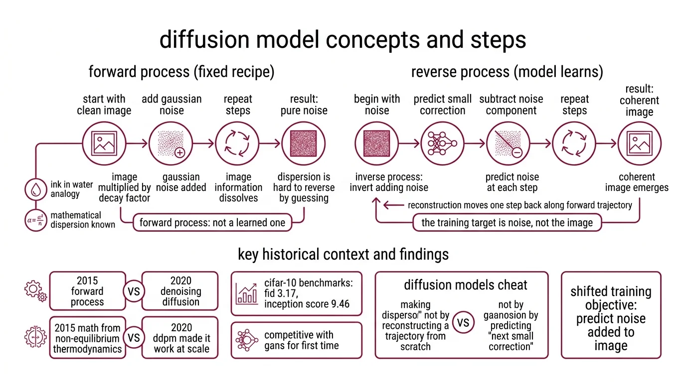
A diffusion model is a generative neural network trained to reverse a fixed noising process. You start with a clean image, add a small amount of Gaussian noise, repeat — and after enough steps the image becomes indistinguishable from pure noise. A diffusion model learns, at each step, to predict the noise that was just added. Do that well enough and you can invert the process: begin with noise, subtract the predicted component, repeat, and a coherent image emerges.

That is the definition. The interesting part is why the training target is the noise rather than the image.

The forward process was first formulated in 2015, borrowing mathematics from non-equilibrium thermodynamics. In 2020, Ho, Jain and Abbeel made it work at scale in “Denoising Diffusion Probabilistic Models,” hitting FID 3.17 and an Inception Score of 9.46 on CIFAR-10 — numbers that made diffusion competitive with GANs for the first time (Ho et al. 2020). What shifted was not the idea. It was the training objective.

The forward process is a fixed recipe, not a learned one

Consider the analogy of ink in water. Drop a bead of ink into a still glass, and within a minute the ink disperses uniformly; information about the original drop dissolves into the solvent. That process is easy to describe mathematically and hard to reverse by guessing. Diffusion models cheat by making the dispersion known. They do not have to reconstruct a forward trajectory from scratch — they have to predict the next small correction that moves one step back along it.

The forward process is a hard-coded Noise Schedule: at each step, the image is multiplied by a small decay factor and Gaussian noise is added. The original DDPM setup used linear betas from 10⁻⁴ to 0.02 over T = 1000 steps (Lil’Log). That schedule is not learned. It is specified up front, and the network never touches it.

What the network learns is the inverse problem. Given a noisy image at step t, predict the noise component. The loss is the mean squared error between the true noise and the predicted noise — ‖ε − ε_θ(x_t, t)‖² (Lil’Log). Clean mathematics, surprising consequences.

How noise prediction becomes image generation

Once you can predict the noise at any step, sampling is mechanical. The forward process is deterministic, the reverse process is a learned approximation, and that asymmetry does most of the work.

How does a diffusion model generate images from random noise?

You start with x_T — a tensor of pure Gaussian noise with the same shape as the target image. At each step, the network predicts the noise component. You subtract a scaled version of that prediction, add a small new perturbation to keep the trajectory stochastic, and move to x_{T-1}. Repeat until you reach x_0. What comes out is a coherent sample from the training distribution.

It helps to think of the latent space as a rugged landscape. Pure noise is a point high on a featureless plateau; the training distribution — the manifold of real photographs — sits in the valleys below. Noise prediction is, roughly, a gradient estimate: which direction leads toward the manifold? The reverse process is a slow descent along that gradient, jittered at each step so the trajectory does not collapse onto the nearest memorised example.

Not magic. A gradient estimate, stepped slowly toward the training manifold.

That analogy is useful for intuition; the strict reading is different. The network does not “undo” the forward trajectory point-by-point. It predicts a quantity — the noise, or equivalently the score, or in newer formulations the velocity — that plugged into an update rule produces a trajectory whose distribution matches the data. “Reverses noise” is a pedagogical shorthand. The effect is reproducible; the literal reversal is not what is happening.

What is the difference between forward and reverse diffusion processes?

Forward: x_0 → x_1 → … → x_T. Gaussian noise is added according to a fixed schedule. No network involved. The conditional distribution at each step has a closed form.

Reverse: x_T → x_{T-1} → … → x_0. The true reverse conditional is analytically intractable for arbitrary data. The network learns a parametric approximation, and because each forward step is small, the reverse step is approximately Gaussian too — which is what makes the approximation tractable at all.

Two consequences matter in practice.

Steps are not symmetric between training and inference. Training uses T ≈ 1000 steps because the Gaussian approximation in the reverse step holds only when each step is small (Lil’Log). Inference does not need all of them. DDIM reformulates the reverse process as non-Markovian and samples in as few as 10–50 steps with comparable quality — the original DDIM paper reports 10× to 50× faster wall-clock inference than DDPM (Song et al. 2020). Rectified-flow models go further, sometimes claiming competitive quality in 1–4 steps, though the exact count depends on the sampler and the task.

Conditioning enters only in the reverse. The forward process has no opinions about what it is destroying; it treats a cat and a cathedral the same. During the reverse pass a conditioning signal — a text embedding, a reference image, a camera motion — steers the gradient. Classifier-Free Guidance is the technique that made text-to-image practical; it jointly trains conditional and unconditional noise predictors and takes a weighted difference at inference, and it is now the de facto standard for text-conditioned diffusion (Ho & Salimans 2022).

Where the architecture goes from here

The original DDPM used a U-Net with skip connections as the noise predictor. That was the backbone for Stable Diffusion 1 and 2, and it still underlies much of the open-source ecosystem. But the frontier has shifted. Pure U-Net backbones are no longer the state of the art.

Diffusion Transformer architectures replace the U-Net with a transformer that operates on patches of the latent representation. Stable Diffusion 3 uses a multimodal diffusion transformer trained with a Rectified Flow objective — a reformulation that learns straighter trajectories between noise and data, which reduces the number of sampling steps needed (Esser et al. 2024). This is the first line of a broader family: Flow Matching reframes diffusion as learning a continuous vector field between distributions rather than a discrete denoising sequence.

The practical effect: in 2026, new frontier models are mostly transformer-based. Veo 3 applies latent diffusion jointly over spatio-temporal video and audio latents, and generates up to 4K at 24 fps with synchronized audio according to the Veo 3 technical report. OpenAI described Sora 2 as a diffusion transformer, though exact architectural details were never published. FLUX.2, released by Black Forest Labs in November 2025, is another transformer-based diffusion system aimed at photorealistic output with multi-reference control.

The U-Net is not going away — it remains efficient for smaller models and mature in tooling — but it increasingly feels like the CNN era of this subfield.

What the mechanism predicts

Once you see diffusion as noise prediction along a learned trajectory, several behaviors stop being mysterious.

• If you give the model more sampling steps, you should observe smoother outputs with fewer high-frequency artifacts, because each step makes a smaller correction and the Gaussian approximation is tighter.
• If you raise the guidance scale in classifier-free guidance, you should observe higher prompt adherence but lower sample diversity, because guidance pushes every trajectory toward the high-probability region of the text-conditioned manifold.
• If you train on a narrow distribution and then sample out-of-distribution prompts, you should observe artifacts that look like interpolations between memorised patterns, not coherent novelty, because the reverse process can only descend toward regions of the manifold it was shown.

Rule of thumb: the network does not draw, it denoises. Sharpness, prompt alignment, coherence, mode collapse — each is a property of the learned noise estimator and the scheduler that consumes it.

When it breaks: diffusion models are expensive at inference because each image requires many sequential network evaluations, and the reverse process cannot be parallelised across steps. A DDIM sampler running in the 10–50 step range still costs that many forward passes per image; video models compound that by the frame count. Aggressive step-reduction techniques — distillation, rectified flow, consistency models — shrink the step count but typically trade off fidelity, diversity, or controllability.

Compatibility notes:

• Backbone shift: The industry is migrating from pure U-Net to Diffusion Transformers (DiT, MM-DiT) for frontier models. U-Net-only tutorials written before 2024 still explain the mechanism correctly, but they cover a narrowing slice of production systems.
• OpenAI Sora 2 availability: Consumer app shutdown was scheduled for April 26, 2026; API shutdown for September 24, 2026. Treat Sora 2 as a transitional example rather than a live reference.

The Data Says

The surprising part of diffusion is not that it works, but that the training target is noise rather than the image. Ho et al. (2020) showed that this reparameterisation made diffusion competitive with GANs on CIFAR-10 at FID 3.17. Six years later, the same idea — predict the noise, descend the gradient, condition along the way — powers essentially every frontier image and video model in production.