What Is a Convolutional Neural Network and How Learnable Filters Extract Visual Features
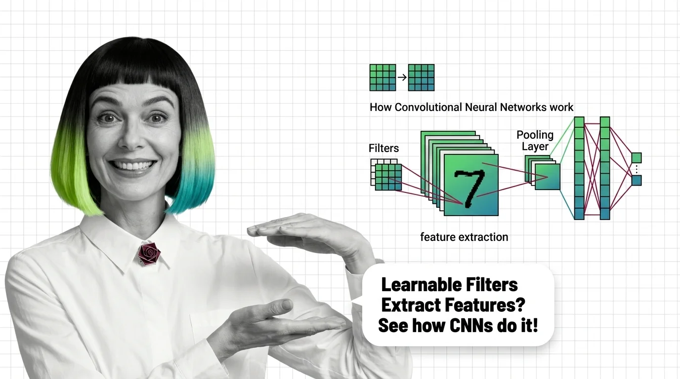
Table of Contents
ELI5
A convolutional neural network slides small number grids called filters across an image, detecting edges, textures, and shapes. Each layer combines simpler patterns into more complex ones — building recognition from raw pixels without explicit instructions.
Train a network to classify a thousand categories of objects — cats, bridges, tumors, galaxies — and something counterintuitive happens in the first layer. The filters don’t learn cats. They don’t learn bridges. They learn edges: horizontal, vertical, diagonal. Every CNN, regardless of dataset, regardless of task, converges on nearly identical edge detectors in its opening layer. The machine reinvents the same geometry every time.
The Geometry a Network Teaches Itself
A standard Neural Network Basics for LLMs treats every input as a flat vector — a 256x256 grayscale image becomes 65,536 independent numbers, each demanding its own weight. No spatial awareness. No concept of adjacency. Convolutional networks reject that premise entirely, and the rejection is what makes them work.
What is a convolutional neural network?
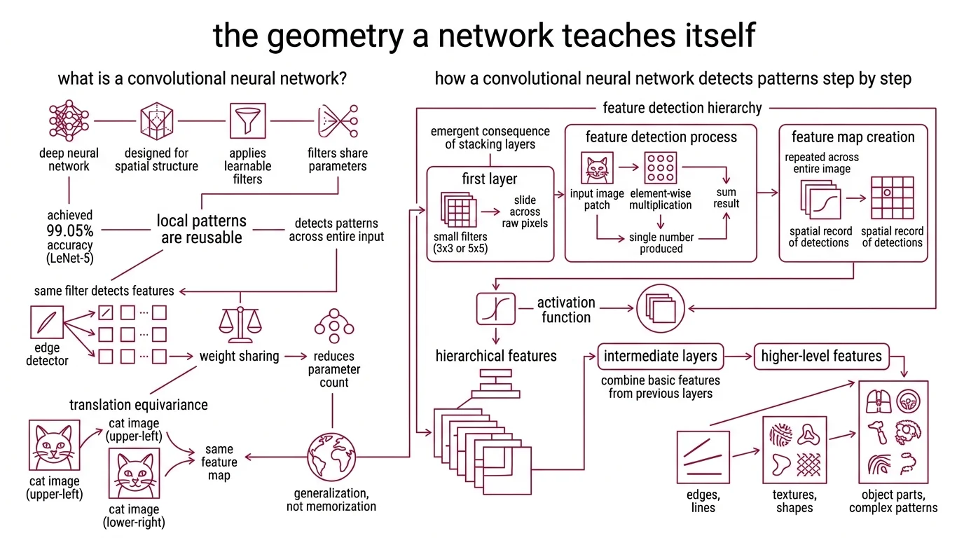
A convolutional neural network is a class of deep neural network designed to process data with spatial structure — images, audio spectrograms, time series — by applying learnable filters that share parameters across the entire input. The original architecture, LeNet-5, was described by LeCun, Bottou, Bengio, and Haffner in 1998 and achieved 99.05% accuracy on handwritten digit recognition (LeCun et al.) — a result that was impressive less for the number and more for the principle it demonstrated.
The principle: local patterns are reusable. An edge detected at position (12, 47) is computed by the same filter that detects an edge at position (200, 3). This mechanism — weight sharing — reduces the parameter count by orders of magnitude while making the network equivariant to translation. A cat in the upper-left corner activates the same features as a cat in the lower-right.
Not memorization. Generalization built into the architecture.
How does a convolutional neural network detect patterns in images step by step?
Detection happens in a strict hierarchy, and that hierarchy is not a design choice — it is an emergent consequence of stacking layers.
In the first layer, small filters (typically 3x3 or 5x5 grids of learnable weights) slide across raw pixel values. At each position, the filter multiplies its weights element-wise with the overlapping image patch, sums the result, and produces a single number. Repeat across the entire image, and you get a feature map — a spatial record of where that particular pattern was detected.
An Activation Function — usually ReLU — then zeros out negative values, keeping only the activated regions. This is where nonlinearity enters: without it, stacking layers would be mathematically equivalent to a single linear transformation, regardless of how deep you build.
The second layer operates on the first layer’s feature maps, not on raw pixels. Its filters detect combinations of edges — corners, junctions, simple textures. The third layer combines those into recognizable parts. By the time you reach deeper layers, the network responds to eyes, wheels, anatomical structures — composite patterns it was never explicitly taught to find.
Each layer builds on the geometry the previous layer extracted. The filters are the only learned component; everything else — the sliding, the summing, the activation — is fixed architecture. What changes between a CNN that reads postal codes and one that detects melanoma is the content of those filters, not the mechanism that applies them.
Anatomy of a Learned Eye
Three distinct layer types divide the labor inside a CNN, and understanding what each one discards is more revealing than understanding what each one computes.
What are convolutional layers, pooling layers, and fully connected layers in a CNN?
Convolutional layers are the feature extractors. Each contains multiple filters — also called kernels — and each filter produces its own feature map. A layer with 64 filters generates 64 parallel views of the input, each tuned to a different spatial pattern (Stanford CS231n). The convolutional layer preserves spatial relationships; it knows where a pattern occurs, not just whether it occurs.
Pooling layers do the opposite: they deliberately destroy spatial resolution. Max pooling takes the highest value from a small window — typically 2x2 — and discards everything else. The destruction is intentional. By reducing spatial dimensions, pooling forces the representation to encode “a vertical edge exists somewhere in this region” rather than “a vertical edge sits at pixel (47, 112).” You gain invariance to small translations at the cost of precise localization.
Fully connected layers sit at the end of the pipeline, where spatial structure has been compressed into a one-dimensional feature vector. Here, the network maps that compressed representation to output classes — “cat,” “dog,” “pneumonia” — using standard dense connections. The spatial information that entered as a three-dimensional tensor exits as a probability distribution over categories.
The progression reveals a clear division: convolutional layers build spatial understanding, pooling layers compress it into portable representations, and fully connected layers make the final classification.
How do filters, feature maps, and activation functions work together inside a CNN?
Think of each depth level as a three-stage cycle.
The filter convolves with its input, producing a raw feature map — a linear response to a spatial pattern. The activation function introduces a decision boundary: ReLU poses a binary question — is this response positive? If yes, preserve it. If no, set it to zero. The activated feature map then becomes the input for the next convolution.
This cycle — convolve, activate, pool, repeat — is the engine that builds the representational hierarchy. Inserting Batch Normalization between convolution and activation stabilizes the entire process by normalizing each feature map’s distribution, so subsequent layers receive inputs with consistent statistical properties. The technique reduced the training steps required for convergence by a factor of fourteen (Ioffe & Szegedy).
Depth matters — and depth creates problems that reveal something important about neural optimization. When He, Zhang, Ren, and Sun pushed this architecture to 152 layers in 2015, they encountered a counterintuitive result: very deep networks performed worse than shallower ones. Not from lack of capacity, but because gradients vanished before reaching early layers. Their solution was the residual connection — a skip path that lets gradients bypass entire layer blocks. The network learns a residual mapping F(x), and the skip connection adds it to the original input: H(x) = F(x) + x. With this mechanism, the 152-layer ResNet achieved 3.57% error on ImageNet (He et al.).
The skip connection didn’t add capacity. It added a survival path for information.
Where the Hierarchy Holds — and Where It Collapses
If the mechanism works by building spatial hierarchies from local patterns, several consequences follow directly.
If your input has strong local correlations — adjacent pixels, neighboring audio frames, sequential sensor readings — a CNN extracts meaningful features with far fewer parameters than a fully connected network. The physics of cameras guarantees that nearby pixels are statistically related, which is why CNNs dominate in image-centric tasks.
If your input lacks spatial structure — tabular data, arbitrary feature columns — convolving a filter across it is computationally valid but semantically empty. The architecture’s inductive bias becomes a liability rather than an advantage.
If you need the network to understand global context — the relationship between a face in the foreground and a building in the background — pooling alone will not bridge the gap. The receptive field grows with depth, but slowly; a 3x3 filter in the fifth layer sees a larger region than one in the first, but the attention remains fundamentally local.
This is the gap that Vision Transformers exploit. As of 2026, ViTs outperform CNNs on large-scale benchmarks when compute is abundant, while CNNs remain dominant for real-time and edge applications where inference speed and memory constraints matter. Hybrid architectures — convolutional stems feeding transformer encoders — increasingly outperform both pure approaches.
Rule of thumb: If your task has spatial locality and your compute budget is tight, a CNN is the stronger architecture. If you need global attention and have data to match, transformers take over.
When it breaks: CNNs fail when discriminative features are not spatially local — when recognition demands understanding relationships between distant input regions. Each pooling layer discards fine-grained positional information that downstream tasks may need. The mechanism that makes CNNs efficient — local filtering plus spatial compression — is the same mechanism that limits their ceiling.
The Data Says
The convolutional neural network’s power traces to a single architectural bet: local patterns are reusable, and they compose hierarchically. From LeNet-5’s edge detectors in 1998 to ResNet’s 152-layer skip connections in 2015, every major advance has refined that bet without replacing it. The geometry the network teaches itself in the first layer remains the foundation for everything it recognizes in the last.
AI-assisted content, human-reviewed. Images AI-generated. Editorial Standards · Our Editors