What Is a Confusion Matrix and How It Reveals Where Your Classifier Fails
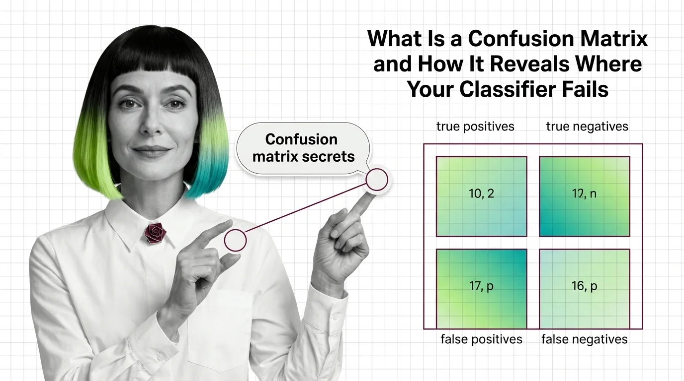
Table of Contents
ELI5
A confusion matrix is a table that sorts every prediction a classifier makes into four buckets — correct positives, correct negatives, and two types of error — so you can see exactly where the model fails.
A fraud detection model scores 99% accuracy on a dataset where barely one in a hundred transactions is fraudulent. The team celebrates. The model goes to production. It catches zero fraud.
The accuracy was real. The performance was an illusion. And the four-cell table that would have exposed the problem in thirty seconds never got built.
The Grid That Exposes a Classifier’s Blind Spots
Think of a confusion matrix as a post-mortem table for every decision a classifier has ever made — not the polished summary on the dashboard, but the raw accounting. Each row represents what actually happened; each column represents what the model predicted. Where rows and columns intersect, you find the truth about your model’s judgment.
What is a confusion matrix in machine learning?
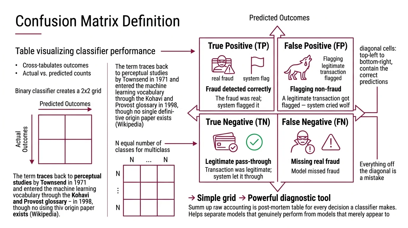
A confusion matrix is a table that visualizes the performance of a classification algorithm by cross-tabulating actual outcomes against predicted outcomes. For a binary classifier, this produces a 2×2 grid. For multiclass problems, it extends to an N×N matrix where N equals the number of classes — each cell C[i,j] counting observations of class i that the model predicted as class j (Wikipedia).
The term traces back to perceptual studies by Townsend in 1971 and entered the machine learning vocabulary through the Kohavi and Provost glossary in 1998, though no single definitive origin paper exists (Wikipedia).
The diagonal cells — top-left to bottom-right — contain the correct predictions. Everything off the diagonal is a mistake. The structure is simple enough to sketch on a napkin, but its diagnostic power is anything but trivial; it separates models that genuinely perform from models that merely appear to.
What are true positives, false positives, true negatives, and false negatives?
Every prediction a binary classifier makes falls into one of four cells, and the confusion matrix gives each its own coordinate:
- True Positive (TP): The model predicted positive, and it was correct. The fraud was real; the system flagged it.
- False Positive (FP): The model predicted positive, but it was wrong. A legitimate transaction got flagged — the system cried wolf.
- True Negative (TN): The model predicted negative, and it was correct. The transaction was legitimate; the system let it through.
- False Negative (FN): The model predicted negative, but it was wrong. Actual fraud slipped through undetected.
The terminology reads like bureaucratic Latin. But the underlying logic is a coordinate system: the first word — true or false — tells you whether the model was right; the second — positive or negative — tells you what the model predicted. Once you internalize that grammar, the matrix becomes readable at a glance.
Here is the critical asymmetry that the matrix makes visible. FP and FN are not equally costly. In medical screening, a false negative (missed cancer) is catastrophic. In email filtering, a false positive (important email in spam) is merely annoying. The confusion matrix forces you to confront which errors your application can tolerate — a question that accuracy alone never asks.
Where Predictions Become Arithmetic
The four cells are not just a bookkeeping device. They are the raw material from which every meaningful classification metric is derived — and the reason those metrics sometimes contradict each other.
How does a confusion matrix evaluate classifier predictions?
The confusion matrix evaluates a classifier by preserving the structure of its mistakes instead of collapsing all predictions into a single score.
Accuracy — (TP + TN) / (TP + TN + FP + FN) — is the ratio this table produces most naturally, and the metric most likely to deceive you. On balanced data, accuracy works. On imbalanced data, it masks systematic failures.
Precision, Recall, and F1 Score emerge directly from different slices of the same table:
- Precision = TP / (TP + FP). Of everything the model flagged as positive, how much was actually positive? Precision penalizes false alarms.
- Recall = TP / (TP + FN). Of everything that was actually positive, how much did the model catch? Recall penalizes missed detections.
- Specificity = TN / (TN + FP). The true negative rate — how well the model identifies what does not belong (Wikipedia, Sensitivity and specificity).
These metrics are not independent dials you can turn freely. Improving precision typically worsens recall as the classification threshold shifts, and the reverse holds just as reliably (Google ML Docs). The confusion matrix makes this tradeoff legible because you can watch the cells shift as you move the threshold — FP drops while FN rises, and you see exactly what you are trading.
The Matthews Correlation Coefficient (MCC) uses all four cells simultaneously and has been described as the most informative single metric derivable from a confusion matrix (Wikipedia). Unlike accuracy, MCC returns a value between -1 and +1 that accounts for all four quadrants; a score of zero means the model performs no better than random guessing, regardless of class distribution.
How to read and interpret a confusion matrix step by step?
Reading a confusion matrix follows a consistent protocol, whether you face a 2×2 binary grid or a 10×10 multiclass table.
Step 1 — Check the diagonal. High values along the diagonal mean the model classifies correctly for those classes. Low diagonal values signal systematic confusion.
Step 2 — Scan off-diagonal cells. Each off-diagonal cell names a specific confusion pair: class A predicted as class B. In a multiclass matrix, the largest off-diagonal values reveal the model’s most common mistakes — and these are rarely random. They often expose semantic similarity between classes that the feature space cannot distinguish.
Step 3 — Compare rows. Each row sums to the total actual instances of that class. A row with most of its mass off the diagonal means the model is failing that class systematically — high false negative rate.
Step 4 — Compare columns. Each column sums to the total predictions for that class. A column with heavy off-diagonal mass means the model is over-predicting that class, pulling in instances that don’t belong.
Step 5 — Derive targeted metrics. Compute precision and recall for the specific classes that matter most to your application. The aggregate scores come last, after you understand where the errors cluster.
In scikit-learn (v1.8.0), the matrix is one function call: sklearn.metrics.confusion_matrix(y_true, y_pred), where the output array follows the convention C[0,0]=TN, C[0,1]=FP, C[1,0]=FN, C[1,1]=TP (scikit-learn Docs). For visualization, use ConfusionMatrixDisplay.from_predictions() or .from_estimator() — the older plot_confusion_matrix function was removed in v1.2 and will raise an import error in current versions.
What 99% Accuracy Conceals
The confusion matrix’s deepest value is not in the metrics it produces but in the illusions it destroys.
Consider a dataset with 10,000 samples: 9,900 negative, 100 positive. A model that predicts “negative” for every single input achieves 99% accuracy while detecting zero positive cases. The confusion matrix for this model reads: TN = 9,900, FN = 100, TP = 0, FP = 0. The accuracy formula returns 99%. The recall is zero (Google ML Docs).
Without the matrix, that number looks like success. With the matrix, it is immediately obvious the model learned nothing about the positive class. It memorized the base rate.
This is not a textbook curiosity. Imbalanced classification appears in fraud detection, rare disease screening, manufacturing defect identification, and network intrusion detection — precisely the domains where the cost of a false negative is highest.
If your dataset has severe class imbalance, accuracy becomes unreliable as a primary metric. Use precision and recall — or better, MCC — to evaluate what the model actually learned. If your recall for the minority class sits near zero, the model is likely predicting the majority class by default; the confusion matrix will show an empty TP cell and a full FN cell. If both precision and recall look acceptable but the model still fails after deployment, examine whether the test distribution matches the deployment distribution — Benchmark Contamination can inflate evaluation metrics beyond what real-world performance supports.
Rule of thumb: Never evaluate a classifier with a single number. Build the confusion matrix first, read the off-diagonal cells second, compute aggregate metrics only after you understand where the errors concentrate.
When it breaks: The confusion matrix assumes crisp class assignments — each prediction mapped to exactly one category. For probabilistic outputs, multi-label tasks, or regression problems, the standard matrix either requires an arbitrary threshold (which introduces its own bias) or does not apply at all. Model Evaluation in those contexts demands different instruments: calibration curves, ROC analysis, or rank-based metrics that operate on continuous scores rather than discrete bins.
The Data Says
A confusion matrix is not a metric. It is the diagnostic table from which all classification metrics are computed — and the only representation that preserves the full error structure of a classifier’s decisions. When a model appears to perform well on a single aggregate score, the matrix is where you go to verify whether that score tells the truth. The four cells are the minimum viable audit of any classification system.
AI-assisted content, human-reviewed. Images AI-generated. Editorial Standards · Our Editors