What Is A/B Testing for LLMs and How Controlled Experiments Evaluate Prompt and Model Variants

Something is wrong with the intuition most developers carry into LLM experimentation. They picture A/B testing the way it works in web analytics: split traffic, wait, read the winner. In web experimentation, the only meaningful source of variance is user behavior — hold the stimulus constant and differences in outcomes can be attributed to the treatment. LLM experimentation introduces a second source of variance that this model doesn’t account for: the model itself. The same prompt, routed to the same model, produces different outputs across inference calls whenever sampling is non-deterministic. That additional layer of stochasticity doesn’t just complicate the analysis — it challenges the foundational assumption of controlled experimentation.

When Your Experiment Subject Samples from Itself

The fundamental challenge of A/B Testing for LLMs isn’t traffic routing. It’s that the system under test is itself non-deterministic, and controlled experimentation was designed for deterministic systems.

What is A/B testing for LLMs?

A/B testing for LLMs is the practice of routing production requests across two or more prompt or model variants to measure which configuration produces better outcomes — defined by quality scores, response latency, token consumption, or cost per request.

The definition sounds clean. The epistemological challenge is more interesting.

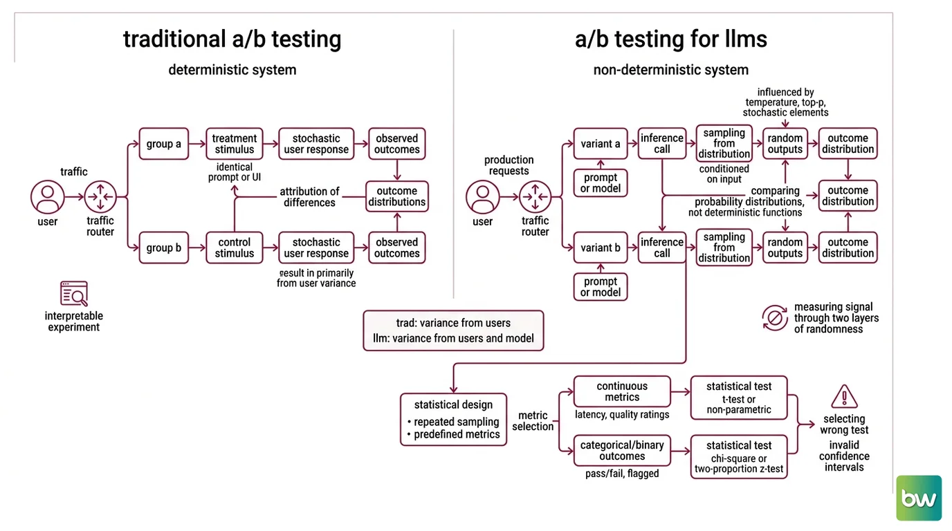
In traditional A/B testing — applied to web interfaces, recommendation algorithms, or email subject lines — any difference in outcome distributions between groups can be attributed to the treatment, because the stimulus is identical within each group and variance comes from the users. That attribution chain is what makes the experiment interpretable.

LLMs dissolve this assumption. Every inference call samples from a probability distribution conditioned on the input. Temperature, top-p sampling, and stochastic elements in the model’s forward pass mean the same prompt produces different outputs across calls. When you compare variant A against variant B, you’re comparing probability distributions, not deterministic functions — and measuring signal through two layers of randomness simultaneously.

Not a technical inconvenience. A statistical design problem.

The industry has converged on methods borrowed from clinical trial methodology: repeated sampling with predefined metrics, using statistical tests calibrated to the metric type. For continuous metrics — latency or quality ratings — a t-test or non-parametric equivalent applies (Statsig Blog). For categorical or binary outcomes such as pass/fail or flagged/not-flagged, a chi-square or two-proportion z-test (Statsig Blog). Selecting the wrong test produces confidence intervals that don’t measure what you think they measure.

From Traffic Assignment to Statistical Verdict

Traffic routing in LLM systems happens at the prompt layer. The infrastructure for getting there is more involved than splitting incoming requests at a load balancer.

How does A/B testing for LLMs work in production?

The most common production pattern uses prompt labels. Teams assign labels — for example prod-a and prod-b — to separate prompt versions and route requests using random assignment in the application layer (Langfuse Docs). Each variant receives an LLM Observability trace tagged with its label. After enough requests accumulate, those traces form the statistical sample for comparison.

Prompt Logging captures what matters: the input, the model output, latency, token count, and any downstream quality signal attached to the request. Latency and Token Budget consumption are automatic. Quality is not, and quality signal is the hardest layer to instrument.

Teams typically approach quality through one of three mechanisms: human raters on a sampled subset, an LLM as a Judge score applied to each response, or a downstream behavioral signal such as task completion rate, escalation to human support, or user correction rate. The behavioral signal is the most informative and the most expensive to define; judge scoring is the most tractable at scale.

Shadow testing warrants a separate treatment from standard traffic splits. In shadow mode, the candidate variant processes real production requests in parallel with the current model — but its output is never served to users. Only the current model’s response reaches the end user. This allows a team to accumulate statistical samples from the candidate without exposing users to potential quality regression. The structural cost is doubled inference spend during the shadow period.

Once Shadow Testing establishes baseline safety, the common pattern is a conservative initial split — starting with as little as 5% of production traffic before scaling wider (Statsig Blog). This mirrors Canary Deployment patterns from infrastructure releases. The goal is identical: catch failures before they affect the majority of users.

Model Routing infrastructure handles the assignment. Whether implemented through feature flag systems, prompt label stores, or dedicated Online Experimentation platforms, the essential requirements are consistency (a given request maps stably to the same variant), logging (the assignment is captured with a unique request ID), and traceability (the assignment can be joined to quality signals days after the request was served).

The Instrumentation Stack

The experiment is only as reliable as the layers underneath it. Every component below must be in place for the statistical output to be interpretable.

What are the key components of an LLM A/B testing framework?

Five components need to be in place for LLM A/B testing to produce actionable results.

1. A versioned prompt store. A reproducible experiment requires knowing exactly which prompt text was served to each request. Prompt Versioning And Management — through tools like Langfuse’s prompt management, MLflow’s prompt hub, or entries in a Model Registry — satisfies this. The version must be immutable at write time and logged at request time.

2. A server-side traffic splitter. The routing logic assigns each request to a variant. The assignment must be stable (so the same request ID doesn’t bounce between variants on retry), recorded with the trace, and applied before the inference call — not after.

3. An observability trace per request. OpenTelemetry provides the standard schema. Distributed Tracing with span-level tagging makes it possible to join downstream quality signals back to the prompt variant that generated them. Without traceable spans, quality scores accumulate with no way to attribute them to a specific variant.

4. A metric collection layer. The four metrics Langfuse tracks per variant — response latency, token consumption, cost per request, and quality eval scores — represent a useful minimum set (Langfuse Docs). Cost per request connects directly to LLM Cost Management decisions: a variant with higher quality scores but substantially higher token consumption is not automatically the right choice.

5. A statistical testing layer. Raw metric averages don’t distinguish signal from noise. The selected test — t-test for continuous metrics, chi-square for binary — produces a p-value and confidence interval. Only when that interval excludes the null hypothesis is the experiment interpretable. Getting the test selection wrong doesn’t just lower confidence — the wrong test invalidates the inference entirely.

Some frameworks add a sixth layer: an automated judge at every request rather than a sampled subset. MLflow’s LLM evaluation, for example, includes an LLM-as-judge scoring step that makes full-volume quality scoring tractable without per-request human review (MLflow LLM Eval).

One constraint worth naming on Prompt Caching: if the inference stack caches prompt prefixes, a cache hit may show artificially low latency relative to a cold inference call. Analysis should either exclude cached requests from latency comparison or stratify cached vs uncached separately to avoid confounding that metric.

A note on tooling: Arize Phoenix integrates with 40+ frameworks including LangGraph and the Claude SDK, and currently operates under the Elastic License 2.0 — not a permissive open-source license (Arize GitHub). Verify the licensing terms match your deployment model before building an internal platform around it.

What the Variance Budget Actually Costs

The instrumentation stack described above has a downstream consequence that catches most teams unprepared.

LLM outputs are noisier than web UI interactions. A user either clicks a button or doesn’t. An LLM response on identical inputs may receive different scores from a judge model across separate inference calls. This output variance means you need substantially more samples per variant to reach the same statistical confidence as a web experiment. More samples means more inference calls — and for reasoning models specifically, repeated sampling for significance is significantly more expensive than for standard instruction-following models, because the compute cost per call scales with the model’s reasoning depth (arXiv 2512.21326).

If a quality score improvement fails to reach statistical significance, the cause is usually one of three things: the improvement is real but the sample is too small; the variants are genuinely equivalent and the observed difference is noise; or the judge model’s own output variance is larger than the signal being measured. The right response to all three is the same — accumulate more samples before acting. Experiment Tracking platforms help by making it possible to accumulate samples across multiple days of production traffic rather than requiring burst synthetic evaluations.

A deeper problem: LLM providers push model updates without version bumps. A model tested against last month may have changed silently in ways the provider did not announce (arXiv 2604.27789). If an experiment runs across such an update, variant A at time T is no longer comparable to variant B at time T+n — the underlying model has changed, confounding the treatment effect. Version-pinning via API parameters, where the provider supports it, or recording the exact model identifier served per request, is the only structural defense against silent provider updates confounding the variant comparison.

Rule of thumb: Start at a conservative traffic percentage and hold it there until the confidence interval stabilizes before expanding to broader coverage.

When it breaks: LLM A/B testing fails when the evaluation metric is misaligned with actual user value — when quality score measures fluency but users care about factual accuracy, or when latency is optimized while downstream task completion rates silently degrade. No traffic splitter corrects for metric misspecification.

The Data Says

A/B testing for LLMs extends controlled experimentation into probabilistic systems — and the probabilistic nature of the output means statistical design matters more, not less. The tooling is mature: prompt labels, versioned stores, observability traces, t-tests, and judge-model scoring. What no tooling provides is a metric that actually measures what your users care about. That problem precedes the experiment, doesn’t resolve during it, and determines whether the winning variant was actually better — or just better-scored.