What Are Similarity Search Algorithms and How Nearest Neighbor Methods Find Matching Vectors
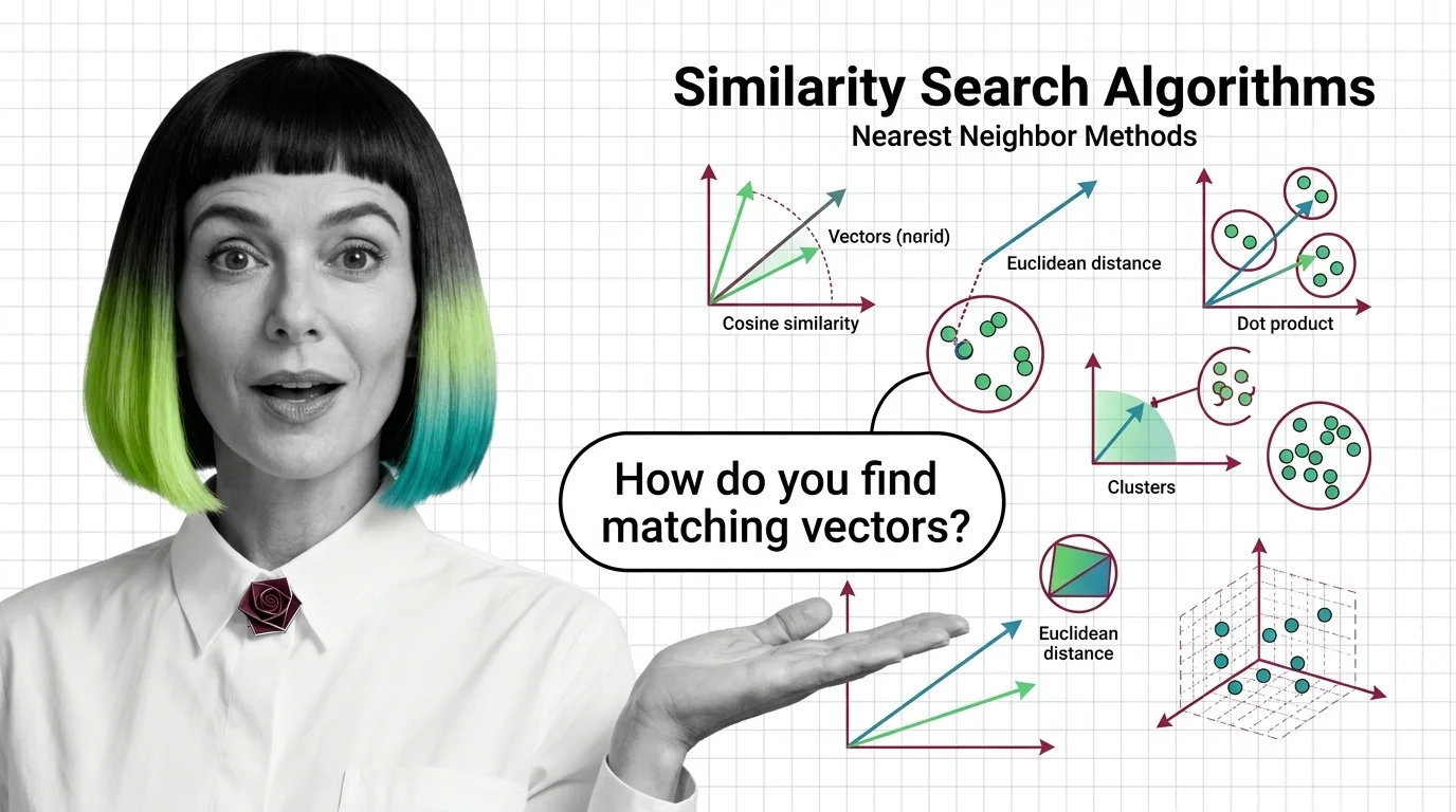
Table of Contents
ELI5
Similarity search algorithms find the closest matches to a query by measuring mathematical distance between vectors — ranking results by geometric proximity instead of keyword overlap.
Here is something that should bother you: two documents can share zero words in common and still be the closest possible match. A Spanish legal brief and an English contract about the same clause will sit nearly on top of each other in vector space — while two English sentences using identical vocabulary can point in opposite geometric directions. The search method that finds one and ignores the other has nothing to do with language. It has everything to do with distance.
The Distance Nobody Told You About
Every modern retrieval system runs on the same quiet assumption — that meaning has a shape, and similar meanings cluster together in geometric space. The mechanism that makes this work is older than transformers, older than deep learning, and far more elegant than most developers realize.
What are similarity search algorithms in machine learning?
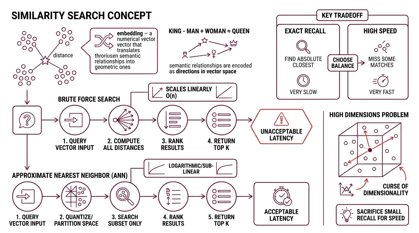
Similarity search algorithms are methods that find the nearest data points to a query in a high-dimensional vector space. The query is an Embedding — a numerical representation where semantic relationships become geometric ones. “King” minus “man” plus “woman” lands near “queen” not because the model understands monarchy, but because the training process encoded that relationship as a direction in space.
The simplest version is brute force: compute the distance between your query vector and every other vector in the dataset, rank, return the top results. For a hundred vectors, this is instant. For a billion, it is suicide.
Not a metaphor. Computational suicide.
Brute-force search scales linearly — O(n) distance computations per query. At the scale of a production embedding index (tens of millions to billions of vectors, each with hundreds of dimensions), a single query would take seconds or longer. Users expect milliseconds. The gap between linear scan and acceptable latency is where approximate nearest neighbor (ANN) algorithms earn their existence.
ANN methods sacrifice a small amount of recall — they might miss the absolute closest vector — in exchange for logarithmic or sub-linear query time. The engineering question is never “exact or approximate?” It is always “how much recall can you afford to lose for how much speed?”
Why Brute Force Dies in High Dimensions
The curse of dimensionality is not a metaphor either; it is a measurable geometric pathology. As dimensions increase, the ratio between the nearest and farthest points from any query converges toward 1.0 — everything becomes approximately equidistant. The geometry that makes search meaningful starts dissolving around the same point where the data gets interesting — hundreds of dimensions, the regime most embedding models operate in.
The algorithms that survive this dissolution work by imposing structure before the query arrives — pre-organizing the vector space so that at query time, most of the space can be ignored.
How does nearest neighbor search work in high-dimensional vector spaces?
Three families of algorithms dominate the field, each exploiting a different structural trick.
Hierarchical Navigable Small World (HNSW) graphs build a multi-layered network where the top layers contain long-range connections (coarse jumps) and the bottom layers contain short-range connections (fine-grained search). A query enters at the top, greedily hops toward the approximate region, then descends layer by layer toward the nearest neighbors. The key insight from Malkov and Yashunin’s original 2016 paper is that this layered structure achieves logarithmic scaling — doubling the dataset size adds one more hop, not twice the work (Malkov & Yashunin). HNSW tends to lead recall-focused benchmarks. It is also memory-hungry; every vector needs graph edges stored alongside it.
Inverted File Index (IVF) partitions the space into Voronoi cells using k-means clustering. At query time, only the vectors inside the nearest cells are searched — typically a small fraction of the total dataset. IVF is the workhorse behind many FAISS configurations (FAISS Docs). The trade-off: cluster boundaries are hard boundaries, and a true nearest neighbor sitting just outside the searched cells will be missed.
Product Quantization (PQ) attacks the problem from a different angle — compression. Instead of searching fewer vectors, PQ makes each vector cheaper to compare. It decomposes the high-dimensional space into a Cartesian product of lower-dimensional subspaces, quantizes each subspace independently, and replaces exact distance computations with table lookups. The original work by Jegou, Douze, and Schmid demonstrated that this approach could compress vectors to a fraction of their original size while retaining competitive recall (Jegou et al.).
In practice, these methods combine. FAISS — developed by Meta FAIR and currently at v1.14.1 — implements IVF+PQ as a standard configuration: IVF narrows the search space, PQ compresses what remains (FAISS GitHub). Locality Sensitive Hashing (LSH) offers another approach entirely, using hash functions that map nearby vectors to the same bucket with high probability, though it has largely been eclipsed by graph-based methods for dense vector search.
Google Research’s ScaNN library takes a related but distinct approach, using anisotropic quantization that gives higher fidelity to directions more likely to affect the ranking order — a detail that explains its strong showing on the ANN-Benchmarks suite (Google Research Blog).
Three Metrics, Three Different Answers
Choosing an ANN algorithm is half the decision. The other half — and arguably the more consequential one — is choosing what “distance” means. Two vectors can be close under one metric and far apart under another. The metric is not a detail; it is a definition of similarity itself.
What is the difference between cosine similarity, Euclidean distance, and dot product for vector search?
Cosine Similarity measures the angle between two vectors, ignoring their magnitude entirely. Two vectors of wildly different lengths pointing in the same direction score 1.0; perpendicular vectors score 0.0; opposite vectors score -1.0. This makes it the default choice for text embeddings where document length should not influence relevance — a 200-word abstract and a 50-page paper about the same topic should be equally “similar” to a query about that topic (Pinecone Docs).
Euclidean distance measures the straight-line distance between two points in vector space. Unlike cosine similarity, it is sensitive to magnitude — a vector scaled by a factor of ten is now “far away” from its original, even though it points in the same direction. This matters when magnitude carries information: in recommendation systems, a user embedding with higher magnitude might represent stronger preference.
Dot product is influenced by both magnitude and direction. On normalized vectors (unit length), dot product and cosine similarity produce identical rankings. On unnormalized vectors, dot product rewards both alignment and magnitude — which can be useful or catastrophic, depending on whether your embedding model was trained with that expectation.
The critical rule: match the metric to the model’s training loss (Pinecone Docs). An embedding model trained with cosine similarity loss encodes information in angular relationships. Searching those embeddings with Euclidean distance introduces a signal (magnitude) that the model was explicitly trained to ignore. The search will return results. They will be wrong in ways that are difficult to diagnose because they look plausible.
| Metric | Sensitive to Magnitude | Range | Best For |
|---|---|---|---|
| Cosine similarity | No | -1 to 1 | Text embeddings, normalized vectors |
| Euclidean distance | Yes | 0 to infinity | Spatial data, magnitude-meaningful embeddings |
| Dot product | Yes | -infinity to infinity | Recommendation, unnormalized with magnitude signal |
When Geometry Meets Your Data
If you switch from cosine similarity to Euclidean distance without renormalizing your vectors, expect retrieval quality to degrade — not because the algorithm failed, but because you changed the definition of “close” without telling the index.
If you see recall dropping as your dataset grows past the IVF cluster count, you are likely under-partitioning. Increasing nprobe (the number of clusters searched) recovers recall at the cost of latency.
If HNSW memory consumption is pushing you toward quantization, expect a recall-compression trade-off — PQ at aggressive compression levels will lose fine-grained distinctions that matter for highly similar items, like legal clauses or near-duplicate code snippets.
Rule of thumb: Start with the metric your embedding model was trained on. If you don’t know, assume cosine similarity — most text embedding models default to it. Verify by testing retrieval quality on a held-out set before trusting it at scale.
When it breaks: Approximate search fails silently. Unlike keyword search that returns obviously wrong results, ANN returns results that look reasonable but are subtly off — the fifth-best match instead of the best, or a semantically adjacent but factually wrong passage. The failure mode is not “no results” but “confident wrong results,” which is harder to catch and more expensive to debug.
Security & compatibility notes:
- pgvector HNSW Buffer Overflow: A buffer overflow vulnerability (CVE-2026-3172) in pgvector versions 0.6.0-0.8.1 allows data leaks or crashes during parallel HNSW index builds. Upgrade to a patched version before running parallel index operations.
The Data Says
Similarity search algorithms convert the abstract problem of “what matches this?” into a geometric one — and the geometry is entirely determined by your choice of metric, index structure, and compression trade-offs. The math is stable and well-understood; the engineering failures come from mismatched metrics, under-provisioned indexes, and the false confidence that approximate results are exact. Measure recall on your own data before you trust the index.
AI-assisted content, human-reviewed. Images AI-generated. Editorial Standards · Our Editors