What Are Scaling Laws and How Power-Law Curves Predict LLM Performance

In 2022, a 70-billion-parameter model outperformed one four times its size. Not through some architectural trick or proprietary dataset — through arithmetic. Chinchilla, trained with the right ratio of data to parameters, beat Gopher on MMLU by seven percentage points (Hoffmann et al.). That result was not a surprise to anyone who had read the equation.

Not a bigger model. A better-allocated one.

The Curve That Predicts Before Training Begins

The most counterintuitive property of modern neural networks is not that they work — it is that their performance is predictable before you start training. Given a compute budget, you can estimate the final loss to within a narrow margin, provided you know the shape of the curve.

That shape is a Power Law.

What are scaling laws in AI and large language models?

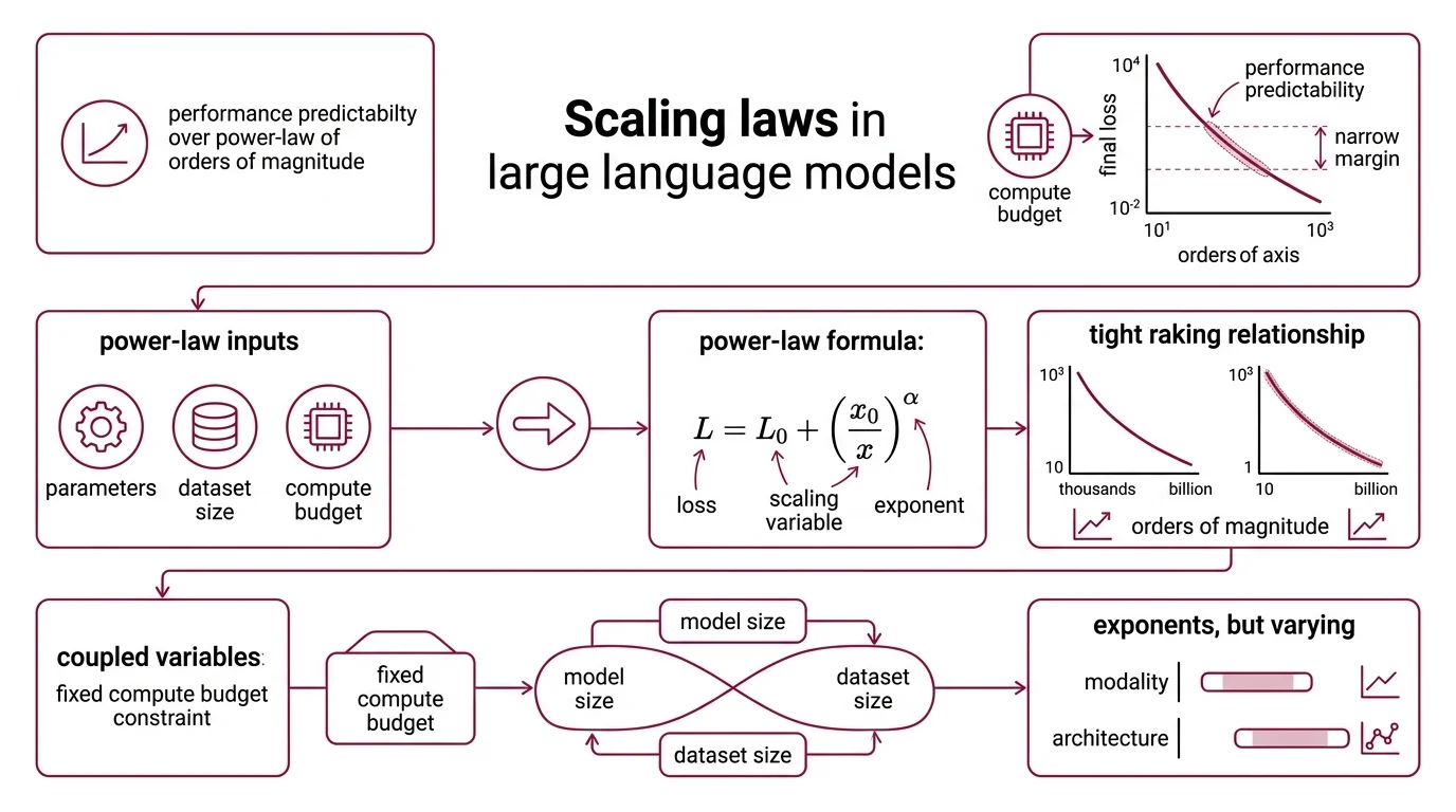
Scaling laws are empirical relationships describing how a model’s Loss Function — the gap between its predictions and correct answers — decreases as you increase one or more of three variables: the number of parameters (N), the size of the training dataset (D), and the total compute budget (C).

The relationship follows a power law: L = L₀ + (x₀/x)^α, where L is the loss, x is the scaling variable, and α is the exponent governing how steeply performance improves. What makes this striking is the regularity. These trends span seven or more orders of magnitude — from models with thousands of parameters to models with billions — with no apparent phase transitions interrupting the curve (Kaplan et al.).

This is not a loose correlation. It is a functional relationship tight enough to guide resource allocation decisions during Pre Training.

But the exponents are not universal. Across modalities and architectures, α ranges from roughly 0.037 to 0.24 for parameter scaling, and 0.048 to 0.19 for compute scaling. The curve’s shape is stable; its steepness depends on what you are measuring and on what architecture you are measuring it in.

How do power-law relationships connect model size, dataset size, and compute budget to LLM loss?

The three variables — N, D, and C — are not independent. They are coupled through a budget constraint: for a fixed compute budget, you must choose how to allocate between a larger model and more training data. Spend too much on parameters and starve the model of examples, and you waste compute. Spend too much on data with a model too small to absorb the patterns, and you waste compute in a different way.

The Chinchilla loss formula makes the coupling explicit: L = A/N^α + B/D^β + L₀, where α = 0.34 and β = 0.28. The first term captures the penalty for insufficient model capacity; the second captures the penalty for insufficient data. L₀ is the irreducible loss — the floor that no amount of scaling will break through.

This decomposition reveals something practitioners often miss: data and parameters do not contribute equally. The exponent on parameters (0.34) is larger than the exponent on data (0.28), meaning — all else equal — adding parameters reduces loss slightly faster than adding data. But “all else equal” is a phrase that collapses the moment you open a real compute budget, because FLOPs constrain both simultaneously.

Three Laws, Three Eras, One Disagreement

Scaling laws are not a single discovery. They are a sequence of corrections, each generation identifying the blind spot in the previous one. Understanding where they disagree tells you more than memorizing any single formula.

What is the difference between Kaplan scaling laws, Chinchilla scaling, and the Densing Law?

Kaplan et al. (2020) established the foundational observation: loss scales as a power law with N, D, and C, spanning seven-plus orders of magnitude. Their practical recommendation was to train larger models on relatively less data, stopping before convergence — if your compute budget is fixed, spend more of it on parameters and less on training tokens (Kaplan et al.).

That recommendation shaped an era. GPT-3 was built on this logic: 175 billion parameters, with the budget weighted toward model size over data.

Hoffmann et al. (2022) — the Chinchilla paper — challenged this directly. Their finding: Kaplan’s approach was not compute-optimal. The correct allocation, they argued, is roughly D ≈ 20N — twenty training tokens per parameter. Under this ratio, both N and D should scale equally with compute: N_opt ∝ C^0.5 and D_opt ∝ C^0.5.

The proof was empirical. Chinchilla, at 70 billion parameters trained on four times more data than Gopher saw, achieved 67.5% on MMLU — seven points above Gopher’s 280 billion parameters (Hoffmann et al.).

A caveat: the D ≈ 20N ratio is debated. Real-world labs — including those training the Llama family — often train on significantly more data than Chinchilla predicts, suggesting the ratio functions as a lower bound, not a prescription.

The Densing Law (Xiao et al., 2025) shifts the lens from absolute scale to efficiency. Published as a cover article in Nature Machine Intelligence, it analyzed 51 open-source LLMs between February 2023 and April 2025, finding that capability density — capability per parameter — doubles approximately every 3.5 months (Xiao et al.). The formula tracks a different curve entirely: ln(N̂/N)_max = At + B, where t is time in days.

Where Kaplan and Chinchilla ask “how big should we build?”, the Densing Law asks “how much capability can we pack into a fixed size?” — a question with immediate consequences for Inference Time Scaling and edge deployment.

One important constraint: the Densing Law was derived from open-source models only. Whether closed-source models follow the same density trajectory remains an open question.

Reading the Exponents

Scaling law papers look intimidating at first encounter — dense with Greek letters, log-log plots, and fit coefficients. But the prerequisites for reading them are narrower than they appear.

What math and machine learning background do you need to understand neural scaling laws?

You need four things, and you can likely skip the rest.

First: logarithmic and power-law functions. Scaling laws are plotted on log-log axes because power laws become straight lines in log space. If you can read a log-log plot and understand that the slope of that line equals the exponent α, you can interpret any scaling curve you encounter.

Second: basic loss-function intuition. Loss is the number a model minimizes during training — typically cross-entropy for language models. You do not need to derive cross-entropy from first principles; you need to understand that lower is better and that the floor (L₀) represents irreducible noise in the data itself.

Third: the concept of compute budgets and the trade-off between model size and data. This is engineering intuition more than formal math — understanding that FLOPs are finite, and every architectural choice is an allocation decision.

Fourth: familiarity with Emergent Abilities and the observation that some capabilities appear only above certain scale thresholds. This is where scaling laws connect to practical ML: the curve predicts average loss, but specific capabilities — reasoning, code generation, few-shot learning — may emerge discontinuously rather than smoothly.

You do not need differential equations, advanced information theory, or deep fluency in optimization algorithms. The foundational scaling law papers are readable with undergraduate-level probability and comfort with exponents.

Where the Power Law Bends

The temptation is to extrapolate — to assume the curve continues forever in the same direction, at the same rate.

It does not.

Predictable linear scaling appears in only 39% of downstream tasks studied; the remaining 61% show irregular behavior — inverse scaling, nonmonotonic patterns, or noise that resists any simple fit (ACL 2025). The power law describes pre-training loss reliably. It describes downstream task performance poorly.

If you are training a foundation model and optimizing for perplexity, scaling laws are your most reliable planning tool. If you are evaluating whether that model will perform well on a specific task after Fine Tuning or RLHF, the curve offers limited guidance — you will need empirical evaluation at the target scale.

There is also the question of diminishing returns. Late 2024 reports indicated that pre-training scaling alone was approaching practical ceilings, prompting labs to explore inference-time compute and data quality as complementary strategies. Inference-time scaling — exemplified by models like OpenAI’s o3 — applies dramatically more compute at the point of use: o3 on high settings consumes 172 times more compute than on low settings, processing 57 million tokens per question versus 330 thousand (NVIDIA Blog). Inference demand is projected to exceed training demand by a factor of 118 by 2026.

When it breaks: Scaling laws predict aggregate loss on the training distribution, not performance on any specific downstream task. A model that follows the predicted loss curve perfectly can still fail on tasks requiring reasoning patterns underrepresented in training data — the curve gives you the average, not the variance.

Rule of thumb: Trust the scaling curve for pre-training budget decisions; verify empirically for any specific downstream capability.

The Data Says

Scaling laws are among the most robust empirical findings in modern machine learning — and among the most frequently over-extrapolated. The power-law relationship between compute, data, parameters, and loss holds across orders of magnitude for pre-training. But downstream, in the tasks that actually matter to practitioners, the majority of scaling behavior is irregular. The curve is real. The extrapolation is a bet.