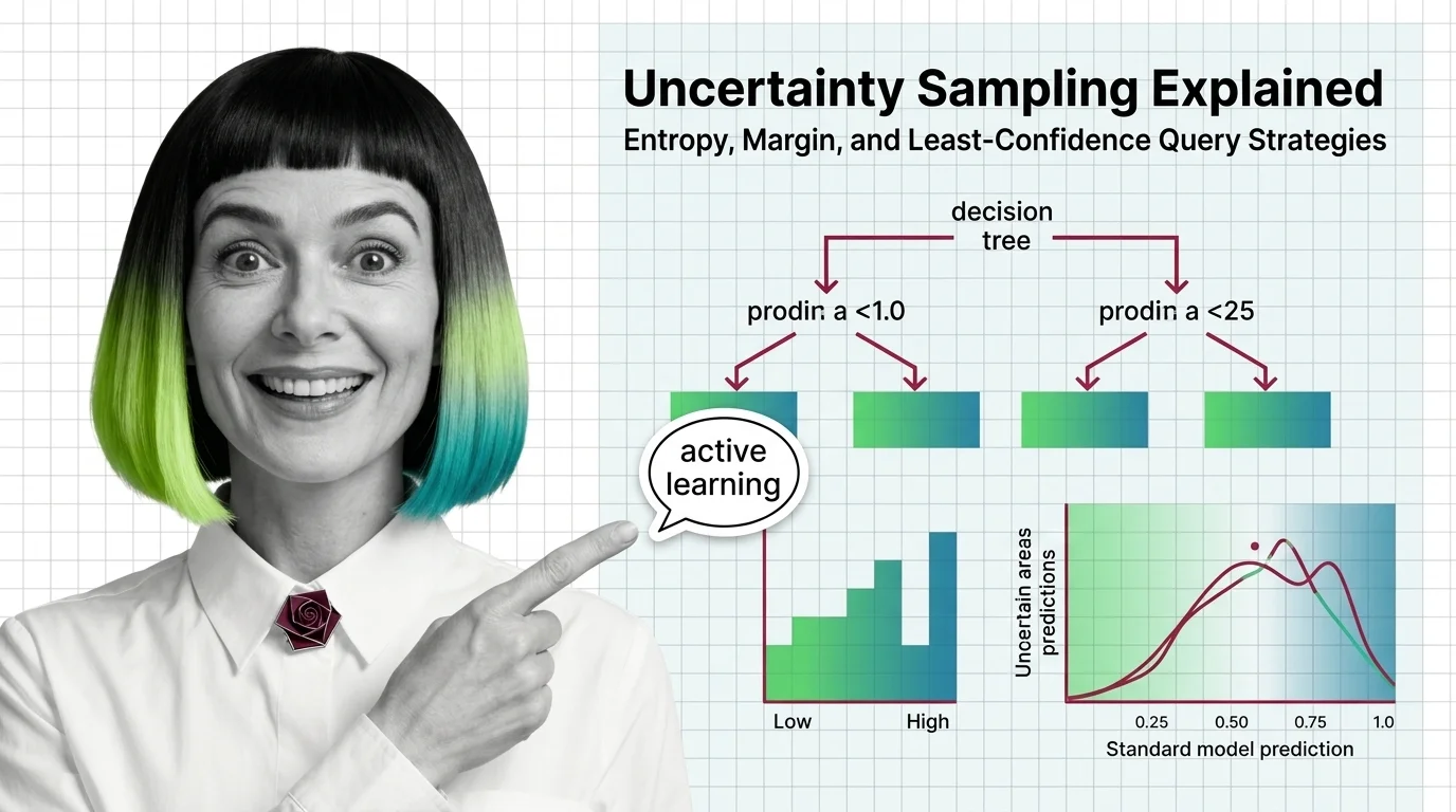
Uncertainty Sampling Explained: Entropy, Margin, and Least-Confidence Query Strategies
ELI5
Uncertainty sampling lets a model choose its own training examples — the ones it’s least sure about. Instead of labeling data at random, you label only what confuses the model most, cutting how much you label.
Two teams label data for the same classifier. One labels ten thousand examples picked at random. The other labels a few hundred — but each one is an example the model was visibly unsure about. The second team’s model wins. That result feels backwards until you look at what a random sample actually contains: mostly examples the model already gets right, which teach it nothing.
This is the central wager of Active Learning: a model is not a passive recipient of training data. It can point at the examples that would teach it the most, if you know how to ask. Uncertainty Sampling is the oldest and most-used way of asking.
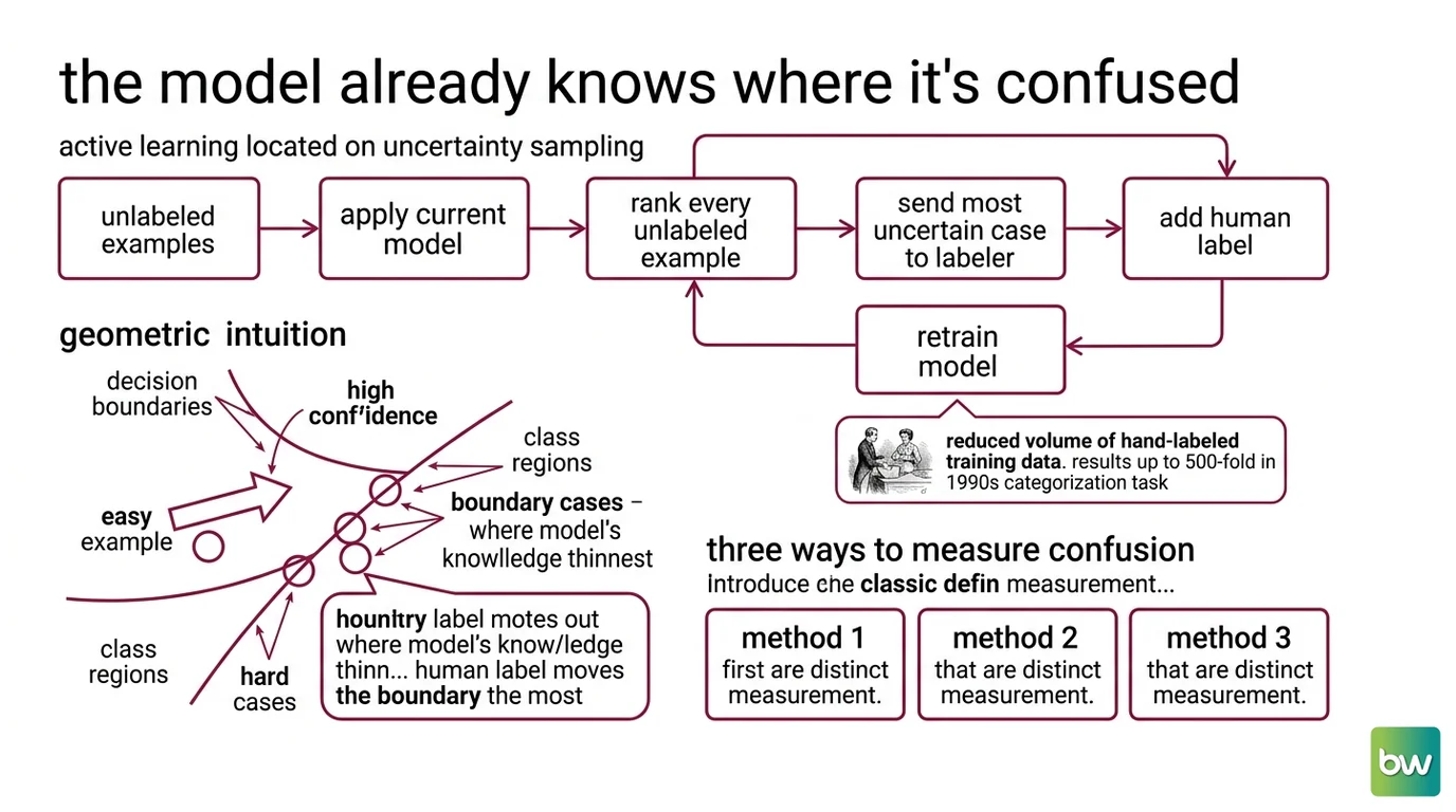
The Model Already Knows Where It’s Confused
A trained classifier doesn’t just output a label. It outputs a probability distribution over labels — a confidence profile for every input. Most pipelines throw that profile away and keep only the top answer. Uncertainty sampling keeps it, because the shape of that distribution is a map of the model’s own ignorance.
What is uncertainty sampling in active learning?
Uncertainty sampling is a Query Strategy: a rule for deciding which unlabeled example a model should ask a human to label next. The rule is simple to state. Rank every unlabeled example by how unsure the current model is about it, then send the most uncertain one to a labeler. Add the new label, retrain, repeat.
The mechanism rests on a geometric intuition. A classifier carves the input space into regions, one per class, separated by decision boundaries. Examples sitting deep inside a region are easy — the model is confident, and a label there confirms what it already believes. Examples sitting near a boundary are the hard cases, where a small shift flips the prediction. Those boundary cases are where the model’s knowledge is thinnest, so a human label there moves the boundary the most.
The idea is old and the early evidence was dramatic. On a 1990s newswire categorization task, Lewis and Gale reported reducing the volume of hand-labeled training data by up to 500-fold to reach a given level of effectiveness (Lewis & Gale 1994). Treat that as an illustrative historical result for one text task, not a number you should expect to reproduce — but the direction it points has held up for three decades.
This raises the obvious question. “Most uncertain” sounds intuitive, but a probability distribution can be uncertain in more than one way. You need a number.
Three Ways to Measure Confusion
There is no single definition of uncertainty. There are three classic ones, and they agree more often than they disagree — until they don’t. Each turns the model’s probability distribution into a single score you can sort by. The canonical reference for all three is Burr Settles’ active-learning survey (Settles Survey).
How do entropy, margin, and least-confidence sampling decide which samples to label?
Least confidence looks only at the top prediction. It picks the example whose most-likely label has the lowest probability — formally, x* = argmin P(ŷ|x). If the model’s best guess on one image is “cat” at 51%, and its best guess on another is “dog” at 94%, least confidence flags the first. The logic: when even your top answer is shaky, you’re guessing.
Margin sampling looks at the top two. It picks the example with the smallest gap between the first- and second-most-likely classes. A 51% top guess with a 49% runner-up is a near-tie — the model is one whisker away from changing its mind. A 51% top guess whose runner-up sits at 10% is far less ambiguous, even though the top probability is identical. Margin captures the part least confidence ignores: how close the competition is.
Entropy sampling looks at the whole distribution. It picks the example with the highest predictive entropy, x* = argmax −Σ P(y_c|x) log P(y_c|x). Entropy is maximized when probability is spread evenly across many classes, so it rewards examples where the model is diffusely confused across the entire label set, not just torn between two options.
| Strategy | What it reads | Flags an example when |
|---|---|---|
| Least confidence | Top class only | The single best guess is weak |
| Margin | Top two classes | The top two are nearly tied |
| Entropy | Full distribution | Confusion is spread across many classes |
Here is the detail that matters in practice. For binary classification, all three strategies are identical — with only two classes, a weak top guess, a narrow margin, and high entropy are the same event. They diverge only when you have three or more classes. There, entropy weighs every class while margin attends to just the top two, so they can disagree about which example is “most” uncertain (Settles Survey). The choice between them is a choice about which kind of confusion you care about.
Where the Questions Come From
The three measures above answer how informative is this example. They say nothing about how the examples reach the model in the first place. That second axis is a separate design decision, and conflating the two is the most common source of confusion in this corner of the field.
What is the difference between pool-based, stream-based, and query-by-committee sampling?
The honest answer is that these three things live on two different axes — and lumping them together hides the structure.
Pool-based sampling and stream-based selective sampling are scenarios: they describe how candidate examples are presented to the learner. In the pool-based scenario, you hold a large fixed pool of unlabeled data, score every instance with your uncertainty measure, rank them, and pick the best to label. It assumes you can see all candidates at once. In the stream-based scenario, instances arrive one at a time, and the learner must decide on the spot whether each one is worth querying or should be discarded — no global ranking, because you never hold the whole set (Settles Survey). Pool-based fits a static dataset you already own; stream-based fits a live feed you can’t store in full.
Query By Committee, by contrast, is a strategy — a different way of measuring uncertainty altogether, and it works in either scenario. Instead of reading one model’s probability distribution, you train a committee of competing models on the same labeled data and ask them all to vote. The example you query is the one they disagree about most, measured by vote entropy or KL divergence between their predictions. The principle, introduced by Seung, Opper and Sompolinsky, is maximal disagreement: where competent models trained on the same evidence still split, the data is genuinely ambiguous (Seung et al. 1992).
So the clean mental model is two questions, not one. How are candidates presented? — pool or stream. How do you score informativeness? — single-model uncertainty (least confidence, margin, entropy) or committee disagreement. Modal Active Learning extends the same two-axis thinking to settings where the candidates are images, audio, or multimodal inputs rather than tidy feature vectors.
Not a single ladder of methods. Two independent dials.
What This Predicts About Your Labeling Budget
The geometry isn’t just an explanation — it makes predictions you can act on before you spend a labeling dollar.
- If your model is genuinely uncertain near the true decision boundary, uncertainty sampling should beat random labeling, and the gap should widen as labels get expensive.
- If you have more than two classes and you switch from margin to entropy, expect the queried examples to shift toward broadly-confused inputs rather than two-way ties — useful when many classes look alike.
- If the same near-boundary examples keep getting queried over and over, your measure is fixating on a narrow region, and you should pair it with Diversity Sampling to cover the input space.
This connects directly to Training Data Quality. Uncertainty sampling is a quality strategy disguised as a quantity one: it doesn’t just label less, it spends the Data Labeling And Annotation budget — the scarce Human In The Loop hours — where a human judgment carries the most information.
Rule of thumb: For two classes, pick whichever measure is easiest to compute — they’re the same. For three or more, use entropy when all classes matter and margin when you mostly care about the closest call.
When it breaks: Uncertainty sampling trusts the model's confidence, so it fails when that confidence is itself unreliable. A poorly calibrated model that is confidently wrong will report low uncertainty on exactly the examples it most needs labeled, steering you away from its real blind spots. It also struggles at the Cold Start Problem: with almost no labels, the early model’s uncertainty estimates are noise, and the first queries can be worse than random.
The Strategy Is Only as Honest as the Probabilities
There’s a deeper point hiding in the failure mode. Every uncertainty measure here is a function of the model’s output probabilities, and those probabilities are an estimate, not a fact. Modern neural networks are often overconfident — they assign high probability to predictions that are wrong at a rate their confidence doesn’t justify. Uncertainty sampling inherits that flaw directly. This is why calibration and committee disagreement matter: a committee can be uncertain even when each individual member is falsely sure, because the disagreement lives between the models, not inside any one of them. The measure you trust should match how much you trust the probabilities underneath it.
The Data Says
Uncertainty sampling works because a trained model’s probability distribution is a usable map of its own ignorance, and the examples near a decision boundary are the ones a human label moves the most. The three classic measures — least confidence, margin, and entropy — collapse into one for binary problems and diverge only with three or more classes. Keep the two axes separate: pool-based and stream-based describe how candidates arrive; least confidence, margin, entropy, and query-by-committee describe how you score them.
AI-assisted content, human-reviewed. Images AI-generated. Editorial Standards · Our Editors