U-Net, VAE, Schedulers, and Text Encoders: The Anatomy of a Modern Diffusion Model

Open the weights of a modern text-to-image system and you will not find “the model.” You will find several specialized networks wired together, each solving a different mathematical problem. The interesting part is that the component doing what most people would call “generating the image” never actually touches a pixel.

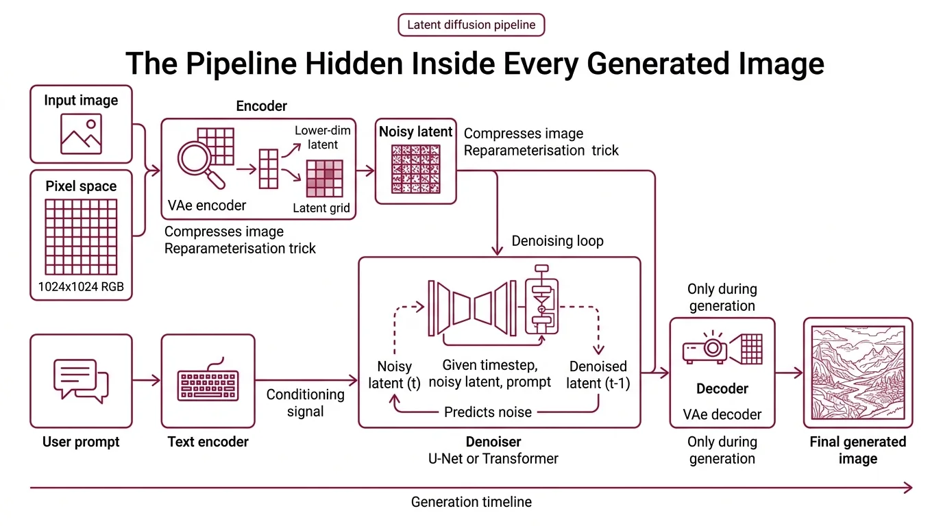
The Pipeline Hidden Inside Every Generated Image

The trick of modern Diffusion Models is that they do almost no work in pixel space. A 1024-by-1024 RGB image is a three-million-dimensional object; learning a denoising function there is possible but brutally expensive. The architecture everyone now uses — introduced by Rombach and colleagues in the Latent Diffusion paper (Rombach et al.) — pushes the computation into a much smaller latent grid and lets a separate network translate back to pixels only at the end.

What are the main components of a diffusion model?

A modern latent diffusion system has four components that play distinct roles. Each is a standalone neural network with its own training objective; the pipeline is their choreography.

The variational autoencoder (VAE) is the compressor. Its encoder maps an input image from pixel space into a lower-dimensional latent grid and its decoder maps that latent back to pixels. The mathematical foundation is the reparameterisation trick, which lets gradients flow through the stochastic sampling step (Kingma & Welling). During generation, only the decoder runs at the end.

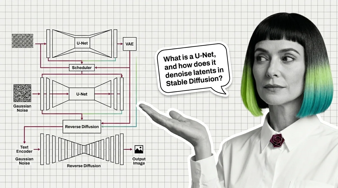
The denoiser is the heart of the system. In the original Stable Diffusion lineage this is a U-Net — a convolutional encoder-decoder with skip connections, a design borrowed from biomedical image segmentation (Ronneberger et al.). In frontier 2024-2026 models like Stable Diffusion 3 and FLUX.1, it is a Diffusion Transformer operating on latent patches. Its job stays the same across architectures: given a noisy latent and a timestep, predict the noise that was added — or, in rectified-flow systems, the velocity toward the data.

The text encoder turns a prompt into a conditioning signal that the denoiser can attend to. SD1.x used CLIP; SDXL stacked CLIP-L with OpenCLIP-G; Stable Diffusion 3 adds a T5-XXL encoder of roughly five billion parameters alongside its CLIP models (Esser et al.). The encoder never generates anything — it produces embeddings that cross-attention layers inside the denoiser consume.

The sampler (also called the scheduler) is not a neural network at all. It is a numerical algorithm that decides how to walk from pure noise to a clean latent: how many steps, what size, and whether the underlying process is interpreted as a stochastic differential equation or an ordinary one. Classifier-free guidance adds a wrinkle: each denoiser step typically runs twice, once with the prompt and once without, with the two noise predictions blended (Ho & Salimans).

Inside the Denoiser — Why U-Net, and Why Not

The denoiser is where the architectural debate of the last two years has played out. Understanding why the original choice was U-Net, and why the frontier has moved, requires looking at what the network is actually being asked to do at each step.

What is a U-Net and how does it denoise latents in Stable Diffusion?

A U-Net has two halves that mirror each other. The contracting path downsamples the input through a sequence of convolutional blocks, each halving spatial resolution while doubling channel depth. The expanding path reverses the process. The signature feature — the one that gives the architecture its name — is the set of skip connections that bridge matching levels, concatenating the encoder’s feature maps into the decoder at equal scale (Ronneberger et al.).

For diffusion, this shape is almost suspiciously well-suited. The noise the network predicts at any timestep lives at every spatial scale — low-frequency noise corrupts global structure, high-frequency noise corrupts local detail. The contracting path gives access to global context; the expanding path emits predictions at full resolution; the skip connections mean local detail is not lost through the bottleneck. Add ResNet-style residual blocks and cross-attention layers that consume the text encoder’s embeddings, and you have the Stable Diffusion U-Net (Rombach et al.). Each denoising pass is the same recipe: noisy latent in with its timestep, text embeddings cross-attended at multiple scales, noise prediction out.

The frontier shift is worth naming precisely. As of 2026, most new large-scale text-to-image models have replaced the U-Net with a transformer backbone — Peebles and Xie’s Diffusion Transformer established that attention scales more predictably than convolutional U-Nets at high parameter counts, and SD3’s MMDiT backbone extends this with separate attention weights per modality joined for a shared attention step (Esser et al.). U-Net is not deprecated — SDXL and its fine-tune ecosystem remain heavily used for ControlNet, LoRA, and specialized domains — but the dominant scaling pattern has moved.

The Sampler Problem — Turning a Continuous Process Into Discrete Steps

The denoiser learns a continuous vector field. The sampler has to integrate it in a finite number of steps. Every choice people argue about on forums — DDIM versus DPM++, Euler versus Heun, Karras sigmas or not — is a choice about numerical integration.

How do schedulers and samplers like DDIM, DPM++, and Euler affect diffusion output?

The training objective of a Denoising Diffusion Probabilistic Models system defines a reverse process over many noise levels — the original DDPM used a thousand Markov steps, each adding a small Gaussian increment (Ho et al.). Sampling that many steps for every image is untenable, so every production sampler is an approximation: a way to take big jumps through the same distribution while preserving quality.

DDIM was the first influential shortcut. Song and colleagues showed that the DDPM training objective is compatible with a non-Markovian reverse process that can be simulated in far fewer steps with the same network (Song et al.). In the Diffusers library, this is DDIM, and it remains the reference point against which other samplers are measured. The training does not change; only the integration does.

Euler and Heun samplers treat the reverse process as an ordinary differential equation over the log-noise level and apply classical ODE solvers. Karras and colleagues systematized this in the EDM framework, arguing that the original DDPM parameterisation conflated several design choices that could be separated; their Heun-based second-order sampler reaches competitive quality at a modest step budget (Karras et al.). DPM-Solver++ takes a different route: it exploits the semi-linear structure of the probability-flow ODE — the drift term admits an exact solution, so only the non-linear part needs numerical approximation — yielding high-quality guided samples in roughly fifteen to twenty steps at paper-reported figures.

The Noise Schedule matters independently of the sampler. A cosine schedule avoids the late-training noise saturation of the original linear schedule, and modern implementations often combine cosine-style schedules with Karras sigmas — a reparameterisation of the noise levels that concentrates steps where the denoiser is most sensitive. Step count, CFG scale, sampler, and schedule are not independent knobs: the same prompt through the same model can produce visibly different images with different samplers, not because the model is less confident, but because the integration trajectory passes through different intermediate latents.

What Math and ML Background This Actually Requires

Before building one of these systems, or before debugging one that misbehaves, the prerequisites stack up in a specific order. Most beginner tutorials skip them; they are also the difference between “I can run a notebook” and “I can reason about why the output looks wrong.”

What math and machine learning background do you need before learning diffusion models?

The prerequisites stack in a specific order. Linear algebra at the level of comfortable tensor reshaping, because skip connections and patch tokens are shape operations on feature maps. Probability at the level where Gaussians, conditional distributions, and KL divergence are familiar — the diffusion framework is phrased entirely in forward and reverse conditionals, and the evidence lower bound is the training objective behind both VAEs and DDPMs (Kingma & Welling; Ho et al.).

Stochastic processes matter at the level of Markov chains and, increasingly, stochastic and ordinary differential equations. The modern view is that the forward diffusion process is an SDE and sampling is numerical integration of its reverse; if terms like “drift coefficient” are unfamiliar, sampler documentation will read as arbitrary. Variational inference is worth singling out — the reparameterisation trick, that sampling z = μ + σ·ε with ε drawn from a standard Gaussian is differentiable in μ and σ, is what makes the whole pipeline learnable end-to-end. Finally, solid intuition for CNNs and attention: the U-Net-to-DiT transition is exactly the swap of one for the other at architectural scale.

The newer formulations deserve a note. Flow Matching and Rectified Flow are closely related but distinct frameworks that generalize and, in some cases, straighten the probability paths classical diffusion uses. SD3 is trained with rectified flow rather than the DDPM objective, and the sampling budget drops because the learned ODE follows straighter trajectories between noise and data (Esser et al.).

What the Architecture Predicts

The four-component structure is not incidental; it is predictive. Once you see the pipeline as distinct networks with distinct failure modes, certain debugging patterns fall out directly.

If you change only the sampler and the composition shifts, the denoiser is doing its job — you have just integrated a different trajectory through the same vector field. If colors look washed out or oversaturated at high CFG, you are seeing classifier-free guidance overshoot: the gap between conditional and unconditional noise predictions is being scaled too aggressively for the sampler’s step size (Ho & Salimans).

If composition is good but fine detail is smeared, suspect the VAE decoder, not the denoiser — the denoiser operates in latent space and cannot produce detail below the VAE’s reconstruction ceiling. If the prompt is ignored selectively — objects present but relationships wrong — suspect the text encoder’s capacity at the relevant conceptual level. SD3’s decision to stack T5-XXL alongside CLIP was explicitly about better compositional understanding in text, not better denoising (Esser et al.).

Rule of thumb: match your sampler’s step budget to your CFG scale, and match your CFG scale to how far from the training distribution your prompt sits.

When it breaks: the most frequent architectural failure is treating the four components as interchangeable. Swapping a SD1.5 text encoder for a SDXL one, or mixing a VAE from one model with a U-Net from another, produces plausible-looking noise at the early steps and collapse by the last step — the components share dimensions but not learned geometries, and no sampler trick recovers what the training did not align.

The Data Says

Modern text-to-image systems are best understood as pipelines of specialized networks, not as single models. The VAE compresses, the denoiser (U-Net or DiT) predicts noise, the text encoder provides conditioning, and the sampler integrates a learned vector field. The frontier has shifted from U-Net to transformer backbones and from discrete-step DDPM to rectified-flow training, but the four-component structure has survived every architectural change since 2022 — because each component is solving a problem the others cannot.