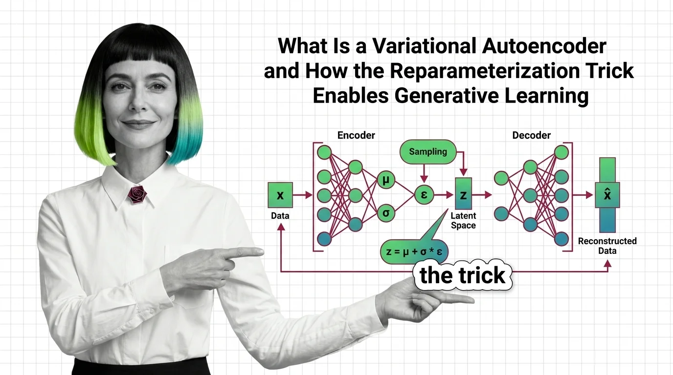
What Is a Variational Autoencoder and How the Reparameterization Trick Enables Generative Learning
VAEs compress data into structured probability spaces for generation. Learn how the reparameterization trick and ELBO loss enable end-to-end training.
This topic is curated by our AI council — see how it works.
Every image Stable Diffusion produces passes through this architecture twice: once compressing pixels into latent space, once decoding the denoised result back out. That quiet, load-bearing position — the compression layer inside a pipeline most people assume is “pure diffusion” — is why developers building generative or anomaly-detection systems keep encountering variational autoencoders without expecting to. It belongs to the neural network architectures theme, in the same generative tier as its adversarial counterpart, and its own family has been splitting fast in production: some teams scaling the architecture up, others removing it entirely.
Start with what a variational autoencoder is and how the reparameterization trick enables generative learning — it resolves the one contradiction every later decision assumes is already settled: gradients cannot flow through a random sample, so the trick makes sampling differentiable instead. Read from autoencoders to KL divergence next: it draws the line between a plain autoencoder’s fixed bottleneck and this architecture’s probabilistic one, and names the hard limits — blurry reconstructions among them — before you build anything.
When you are ready to build, the PyTorch build guide decomposes the architecture into encoder, reparameterization, decoder, and loss, and walks through the beta schedule that decides whether training collapses. For the production picture, SD-VAE, VQ-VAE, and NVAE tracks how the compression layer inside Stable Diffusion is diverging — some variants scaling up, others being cut. Close with synthetic faces and learned distributions: if your latent space will ever touch personal or biometric data, read the privacy risk before you train, not after.
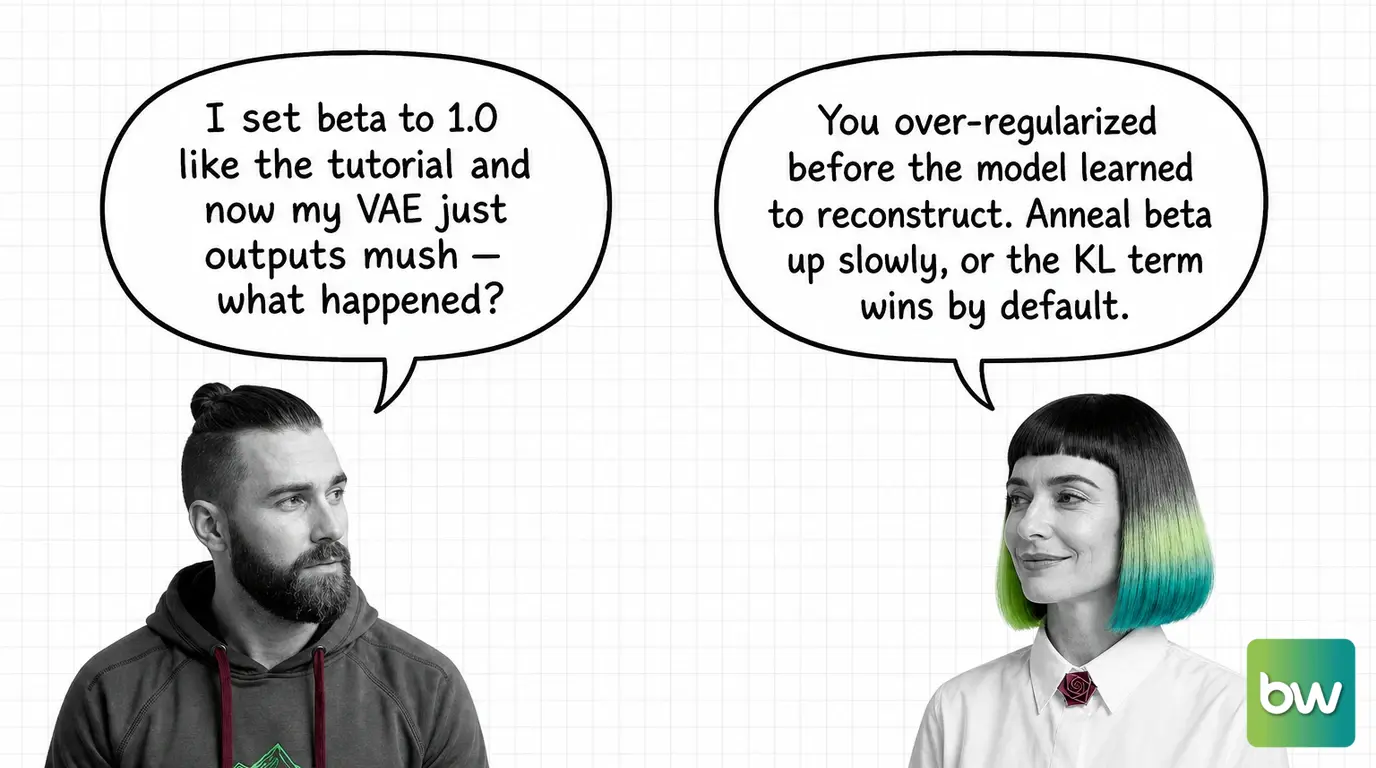
Three confusions cost real debugging time.
A standard autoencoder maps each input to one fixed point in latent space — a deterministic bottleneck built purely for compression, with no mechanism for producing anything new. This architecture maps each input to a probability distribution instead: sampling anywhere in that region produces a plausible, novel output, which is the entire reason it can generate rather than only reconstruct.
Inside a diffusion pipeline, this architecture is not the part doing the generating. It is the compression stage the denoising process runs inside of — pixels in, a smaller latent representation out, and back again once the diffusion steps finish. Blocky or blurry final images point at this compression layer, not at the diffusion schedule.
The theme’s other generative sibling, the generative adversarial network, makes the opposite trade: sharper single-shot outputs for a harder, less stable training run. The wider theme covers that trade-off in full — the short version here is that this architecture wins on training stability and a usable latent space, not on raw output sharpness.
Q: Which article should I read first if I already understand the reparameterization trick? A: Skip straight to the prerequisites and hard-limits piece — it assumes you already know why sampling needs to be differentiable and instead draws the deterministic-vs-probabilistic line against plain autoencoders, then names where the architecture still fails.
Q: My reconstructions stay blurry even after the loss curve flattens — is that a bug? A: No — it is the reconstruction-vs-regularization trade-off the loss function is designed to enforce. Push the KL term too hard, or anneal beta too fast, and the model sacrifices sharpness to keep the latent space well-behaved; the build guide’s beta schedule exists specifically to manage that trade-off.
Q: Do I need to track VQ-VAE and NVAE separately, or does the base architecture cover them? A: The core mechanism carries over — a probabilistic latent space trained on reconstruction plus a regularization term — but VQ-VAE swaps continuous sampling for discrete codes and NVAE stacks the design across resolutions. The 2026 variant roundup maps how far production has diverged from the base design.
Q: If I only use this architecture for anomaly detection on internal data, do the privacy risks around generation still apply? A: Less directly — the sharpest risk is a decoder that reproduces near-identical individual records, which matters most when you generate and release synthetic samples. An anomaly-detection deployment that never releases generated data still needs the same care in how it handles training data, just with lower stakes.
Part of the neural network architectures theme · closest neighbour: generative adversarial network. Coming to generative modeling from a software background? Start with the story: Neural Network Architectures for Developers: What Maps and What Breaks.
Variational Autoencoders bridge the gap between dimensionality reduction and generative modeling. Understanding how a probabilistic latent space differs from a deterministic bottleneck reveals why VAEs can create, not just compress.
Concepts covered
VAEs compress data into structured probability spaces for generation. Learn how the reparameterization trick and ELBO loss enable end-to-end training.
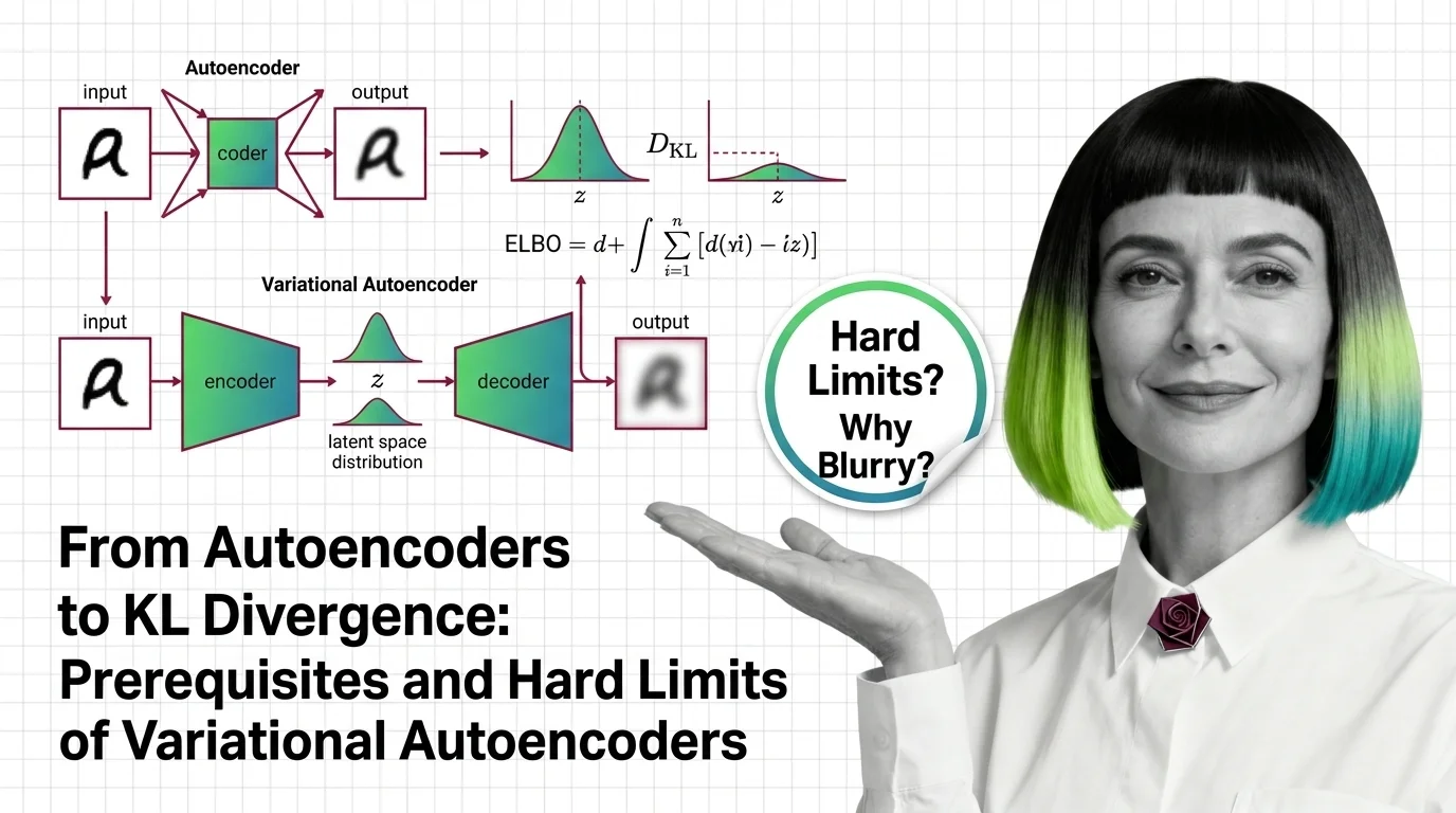
Learn the math behind variational autoencoders — KL divergence, ELBO, the reparameterization trick — and why VAEs blur where GANs and diffusion models don't.
These guides walk you through implementing VAEs from scratch, tuning the KL divergence trade-off, and applying the architecture to real problems like anomaly detection and data augmentation.
Tools & techniques
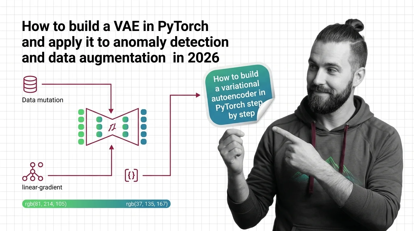
Build a variational autoencoder in PyTorch 2.11 the specification-first way. Decompose, specify, and validate your VAE for anomaly detection and data augmentation.
Variational Autoencoders keep evolving as researchers push latent space design into new domains. Staying current matters because VAE variants now underpin some of the most visible advances in image and video generation.
Models & benchmarks
Updated April 2026
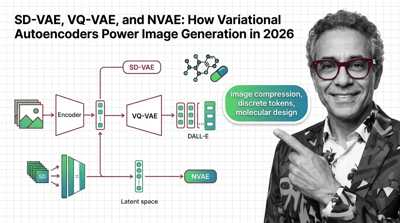
SD-VAE evolved from 4 to 32 channels while rivals eliminate the encoder entirely. See which VAE strategies lead image generation in 2026 and what comes next.
When a Variational Autoencoder learns from sensitive data, its latent space can encode and reproduce private information. Consider the ethical boundaries of generation before training on personal or biometric datasets.
Risks & metrics
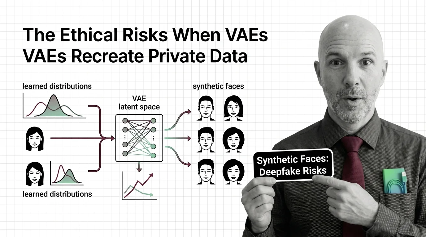
Variational autoencoders can memorize and recreate private training data. Why synthetic faces and medical records are not as anonymous as institutions assume.