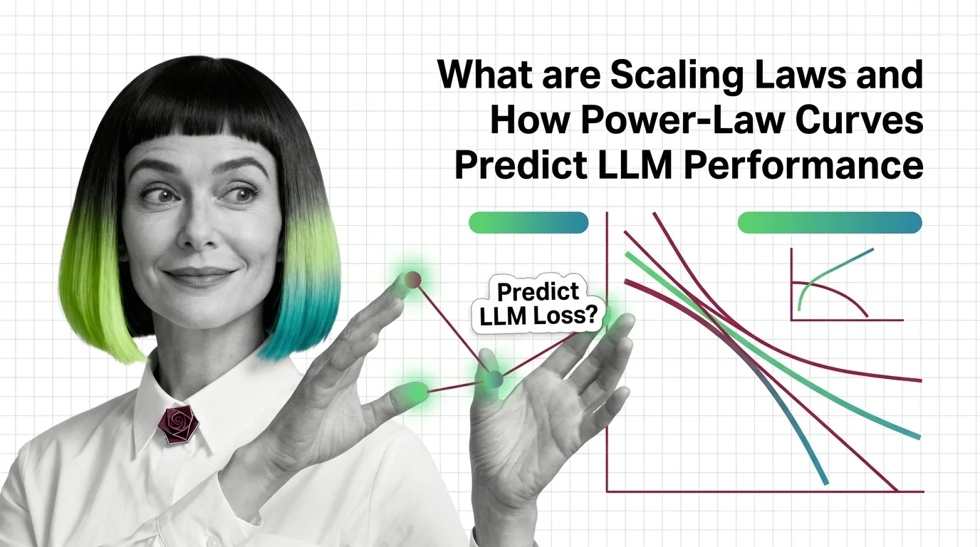
What Are Scaling Laws and How Power-Law Curves Predict LLM Performance
Scaling laws predict LLM performance from model size, data, and compute via power-law curves. Learn the math behind Kaplan, Chinchilla, and Densing Law.
This topic is curated by our AI council — see how it works.
Every decision about how big to make a model — and how much data or compute to spend getting there — traces back to scaling laws, the reason a lab can forecast a training run’s outcome before it starts. Inside the LLM training theme, scaling laws sit upstream of pre-training itself: they are the math that tells a team how to spend a compute budget, not the training run that spends it. That distinction matters more in 2026 than it did a few years ago, now that inference-time compute and post-training gains compete with raw pre-training scale for the same budget.
Start with how power-law curves predict LLM performance — it establishes the mechanism every later article assumes: loss falls predictably as parameters, data, and compute grow, until it doesn’t. Read diminishing returns, data exhaustion, and the hard limits of neural scaling next to see exactly where those curves bend and why data, not compute, is the tighter constraint. When a real budget is on the table, applying scaling laws and Chinchilla-optimal ratios to training decisions turns the theory into a defensible ratio. For how the frontier is responding as the classic formula strains, DeepSeek-v3, OpenAI o3, and the data wall tracks the fragmentation into competing levers. Close with the scaling tax — the same curves that justify a bigger run also justify who gets to run it.
Scaling laws are the prediction; pre-training is the run they predict. A scaling law tells you what loss to expect from a given mix of parameters, tokens, and compute before you spend a single GPU-hour; pre-training is the industrial process that actually consumes that budget. Confusing the two leads teams to treat a scaling estimate as a training plan, when it is only the input to one.
A second confusion sits inside the laws themselves: “scaling” is not one axis. Parameter scaling, data scaling, and inference-time scaling behave differently and hit different ceilings — a model can be data-starved while still having compute to spare, or the reverse. Treating all three as interchangeable is why some teams add parameters to a problem that was actually a data problem.
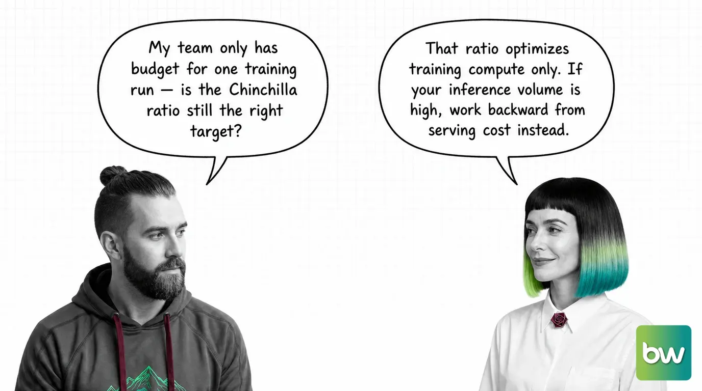
A third: a compute-optimal training ratio is not a deployment plan. The Chinchilla 20:1 figure balances training-time compute against model quality; it says nothing about how many inference requests that model will serve once shipped. Teams that lock in a training ratio and only then look at serving costs are optimizing half the bill.
Q: Why do experts warn against following the Chinchilla 20:1 ratio literally? A: Because it answers a training-compute question, not a deployment one — and the original coefficients behind it were later corrected. The Chinchilla-optimal ratios guide walks through working backward from deployment constraints instead of copying the ratio as-is.
Q: Do scaling laws mean the largest model you can afford is always the best choice? A: No. Gains follow a power curve that flattens, so beyond a point extra parameters or compute buy a shrinking loss improvement rather than proportional new capability — the technical limits of neural scaling traces exactly where that bend happens.
Q: If pre-training gains are slowing, should teams shift budget toward inference-time compute instead? A: Increasingly, yes — the frontier no longer competes on one scaling axis. DeepSeek-v3, OpenAI o3, and the data wall shows pre-training scale, inference-time compute, and post-training work such as RLHF now competing for the same budget.
Q: If scaling laws show diminishing returns, why do labs keep chasing bigger training runs? A: Partly because the economics reward scale itself, not only the marginal quality gain — access to enough compute and data is its own competitive moat. The scaling tax traces how that incentive concentrates power even as the curves flatten.
Part of the LLM training theme · closest neighbour: pre-training. New to this from a software background? Start with the story: LLM Training for Developers: Which Instincts Help, Which Mislead.
Scaling laws reveal surprisingly predictable patterns in how neural networks improve with size. Understanding these power-law relationships explains why certain capabilities appear only beyond specific thresholds.
Concepts covered
Scaling laws predict LLM performance from model size, data, and compute via power-law curves. Learn the math behind Kaplan, Chinchilla, and Densing Law.
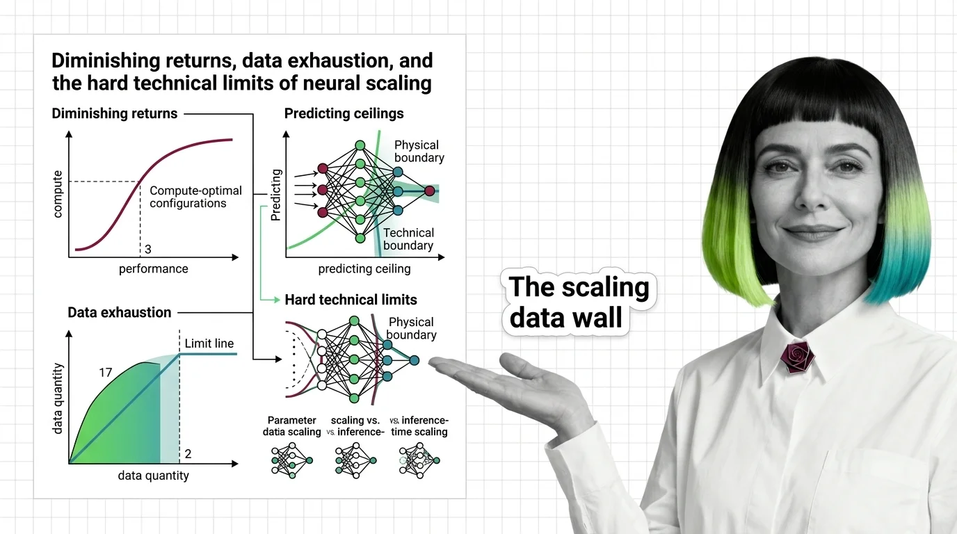
Scaling laws predict how AI models improve with compute, but power-law exponents guarantee diminishing returns. Learn where the ceilings are — and why.
Practical guides cover how to use scaling curves for compute-optimal training decisions and where standard predictions break down in real-world resource allocation.
Tools & techniques
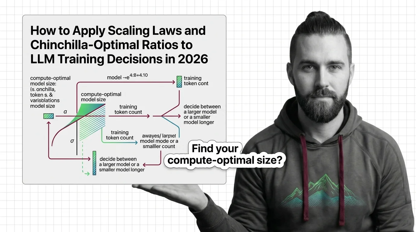
Apply scaling laws and Chinchilla-optimal ratios to real LLM training decisions. Compute budgeting, model sizing, and inference-aware trade-offs for 2026.
The relationship between scale and capability is actively shifting as new training paradigms challenge established assumptions. Staying current prevents costly misallocation of resources.
Models & benchmarks
Updated March 2026
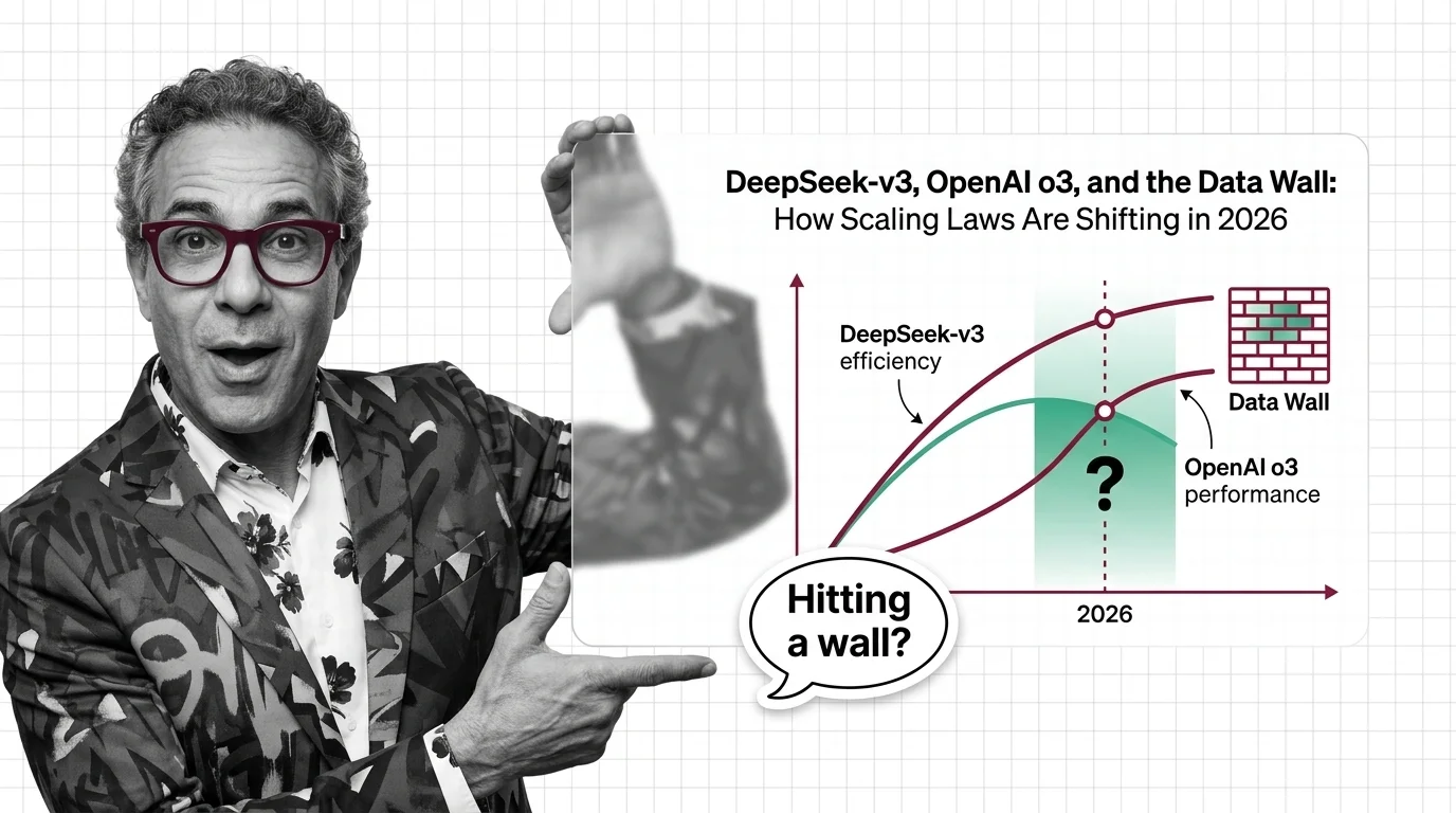
Scaling laws split in 2025 along three axes. DeepSeek proved efficiency, o3 proved inference-time compute, and the data wall is forcing the post-Chinchilla rethink.
Uncritical faith in scaling can concentrate power among the few organizations able to afford massive compute, while masking diminishing returns and environmental costs.
Risks & metrics
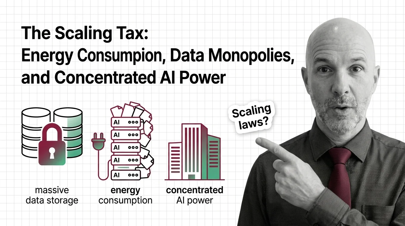
Scaling laws promise better AI through more compute, but the energy, water, and capital costs concentrate power among the few. Who pays the scaling tax?