Diffusion Models in 2026: Slow Sampling and Hard Engineering Limits

FLUX.2 renders a photorealistic portrait in seconds, yet still attaches six fingers to a perfectly lit hand. Stable Diffusion 3.5 will spell COFFEE on a coffee shop sign — and then garble the tagline beneath it. The failures are not random. They are geometric, and they tell you exactly what kind of machine you are using.

Why iterative denoising is diffusion’s physics bill

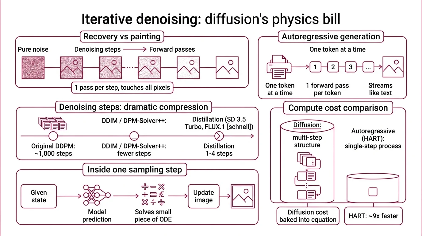
The best way to understand a Diffusion Models system is to watch it fail at speed. Every image a diffusion model generates is not painted — it is recovered. The model starts from pure Gaussian noise and gradually subtracts that noise across many forward passes through a neural network. That “gradually” is where the cost lives.

Why are diffusion models slower than autoregressive image models?

An autoregressive image model predicts one token at a time and streams them out like a language model producing text. One forward pass, one token, no backtracking. A diffusion model does the opposite: every image requires a chain of forward passes over the entire latent — not one pass per token, but one pass per denoising step, with each pass touching every pixel or patch.

The original Denoising Diffusion Probabilistic Models formulation used a thousand sampling steps. Modern pipelines compress that dramatically. DDIM deterministic sampling and DPM-Solver++ cut the count to far fewer steps without visible quality loss. Distillation methods push further: Stable Diffusion 3.5 Large Turbo generates usable images in only four steps (Modal Blog), and FLUX.1 [schnell] ships under Apache 2.0 with a one-to-four step budget (Hugging Face).

But four steps is not one step. Each step is a full forward pass through a model that may be an 8-billion-parameter Diffusion Transformer like SD 3.5’s MMDiT, or the 12-billion-parameter rectified flow transformer inside FLUX.1 [dev]. An autoregressive alternative like HART matches diffusion quality at roughly nine times faster inference by avoiding the multi-step structure entirely (MIT News). The compute cost of diffusion is not a tuning problem. It is baked into the sampling equation.

Inside one sampling step

A single step solves a small piece of an ordinary differential equation. The model asks: given where we are on the path between noise and signal, what direction do we move next? Classical diffusion learned that direction as a denoising score. The 2026 generation learned it as a velocity field — rectified flow, introduced in Liu et al. 2022, teaches the network to follow straight ODE paths from noise to data, which is why a handful of steps can suffice.

The denoiser itself is usually either a U-Net — the legacy encoder–decoder with skip connections that SDXL and earlier pipelines built on — or the transformer-based MMDiT that SD 3 and 3.5 adopted after Esser et al. 2024 demonstrated that rectified flow transformers scaled cleanly with compute. A Noise Schedule governs how much noise sits at each step; the schedule is as much a design choice as the architecture itself, and shifting it changes where the model spends its denoising effort along the path.

Not engineering laziness. Architectural debt.

The step count is not a knob you turn for free — it is the core of what a diffusion model does. Cut the steps too aggressively and the solver overshoots the ODE trajectory, producing the oversaturated, blown-out highlights reviewers have flagged for years.

Where the 2026 frontier still breaks

The open-weights frontier has consolidated around two architectural bets: Stability AI’s SD 3.5 family (8B Large, 2B Medium, and a four-step Large Turbo) and Black Forest Labs’ FLUX line, culminating in the 32-billion-parameter FLUX.2 released in November 2025 (Melies). Both train with rectified flow. Both use transformer backbones. And both still break in roughly the same three places.

What are the biggest technical limitations of diffusion models in 2026?

Three architectural limits keep reappearing across benchmarks.

First, sampling latency — discussed above, and not solvable by scale alone.

Second, Classifier-Free Guidance (CFG) oversaturation. At the high guidance scales users want for prompt adherence, the CFG update vector develops a parallel component that pushes pixel values past the color manifold. The APG paper (arXiv:2410.02416) decomposed this into parallel and orthogonal components, showing the orthogonal part aids image quality while the parallel part causes the burn-out artifacts users see at high CFG scales. A June 2025 follow-up (arXiv:2506.21452) isolated low-frequency information as the primary driver of those artifacts across SD-XL, 2.1, 3.0, 3.5, and SiT-XL. These are research methods, not shipping defaults — the oversaturation is not solved in the production pipelines you are likely using.

Third, a scaling ceiling. A study of scaling laws for diffusion transformers reported power-law FID improvement with diminishing returns above roughly three billion parameters for text-to-image (OpenReview). FLUX.2 at thirty-two billion and the next generation of proprietary models keep improving, but the gains per compute unit flatten in a way that language-model scaling does not. That study was a specific text-to-image setup; the finding should not be generalized to every generative modality, but within this one it is consistent.

Why do diffusion models struggle with text, hands, and fine compositional control?

Because the failure mode is intrinsic to denoising. The denoiser is a local smoother operating on a global constraint problem. Text in an image requires exact spatial arrangement of strokes and spacing. Hands require a precise topology of five fingers with correct joint counts. A prompt like “a red cube to the left of a blue sphere” requires a relational check that spans the whole canvas. Iterative denoising is excellent at locally plausible textures and weak at enforcing discrete, rule-based constraints.

Modern text encoders helped. SD 3’s addition of a T5-XXL encoder alongside CLIP dramatically improved short-text rendering — product logos, single words on signs, short slogans. But multi-line typography, small fonts, and dense layouts still fail. Evaluation frameworks published in 2025 confirmed that multi-object recall, text-in-image accuracy, and location or pose constraints remain weak across the frontier (arXiv Prompt Robustness 2507.08039).

Hands are the canonical tell. FLUX has a consistent reviewer-reported edge over SD 3.5 on hand accuracy — a qualitative consensus, not a quantified benchmark. The edge likely comes from scale and a cleaner training objective, not from any hand-specific architecture. That is the honest version of the story: more parameters and rectified flow make the failure less frequent, but they do not dissolve it.

What the step-count trade-off predicts

If you understand the mechanism, the failure modes stop being mysterious and start being predictable. A few if/then patterns fall directly out of the architecture:

• If you push CFG scale high for prompt adherence, expect oversaturation and clipped highlights — the parallel component of the guidance vector is doing the damage, not your prompt.
• If you drop to four steps or fewer on a distilled model, expect small-detail fidelity to collapse first (text edges, finger topology) while overall composition survives.
• If you scale a pure diffusion transformer past the multi-billion-parameter region on a fixed text-to-image setup, expect FID gains to flatten and compositional errors to persist.
• If the prompt contains multiple objects in explicit spatial relationships, expect relational accuracy to degrade faster than photorealism.

Rule of thumb: Match step count to what you need to be perfect. More steps buy you fine detail; more parameters buy you plausibility, not correctness.

When it breaks: The sharpest failure is compositional. When a prompt demands exact counts, exact positions, or exact text strings, diffusion’s local denoiser cannot enforce those constraints reliably, and no amount of prompt engineering fully patches an architectural limitation. As of 2026, hybrid approaches like HART and autoregressive-first systems such as OpenAI’s GPT image generation are the practical escape hatch, though OpenAI has not fully disclosed the internal architecture and external reverse-engineering suggests an internal diffusion decoder remains in the mix.

The Data Says

Diffusion models in 2026 are faster and more accurate than any prior generation — and still bounded by the same three architectural walls: iterative sampling latency, classifier-free guidance artifacts at useful scales, and weak enforcement of discrete compositional constraints. The 32-billion-parameter frontier does not dissolve these walls. It pushes them back a measured, quantifiable amount.