Sample Size, Statistical Power, and Why Measuring LLM Output Quality Is Harder Than Click-Through Rates

A click either happened or it didn’t. CTR experiments inherit this gift: binary outcomes, stable variance, and enough daily observations to reach significance within hours. LLM output quality offers none of that. It’s continuous, stochastic, context-dependent — and infected by a layer of noise that most evaluation setups never isolate, let alone account for.

Teams that carry web testing intuition directly into LLM evaluation discover the problem empirically. Experiments conclude, results contradict previous experiments, and nobody can explain why. The data volume looks sufficient. The p-values look fine. The conclusions are still wrong.

Not a data problem. A variance architecture problem.

The Variance Nobody Budgets For

Before any A/B Testing for LLMs experiment can answer a meaningful question, you need to know how much noise you’re working through. With LLM quality metrics, the noise has multiple sources — and they compound in ways that don’t announce themselves.

What concepts do I need to understand before running A/B tests on LLM outputs?

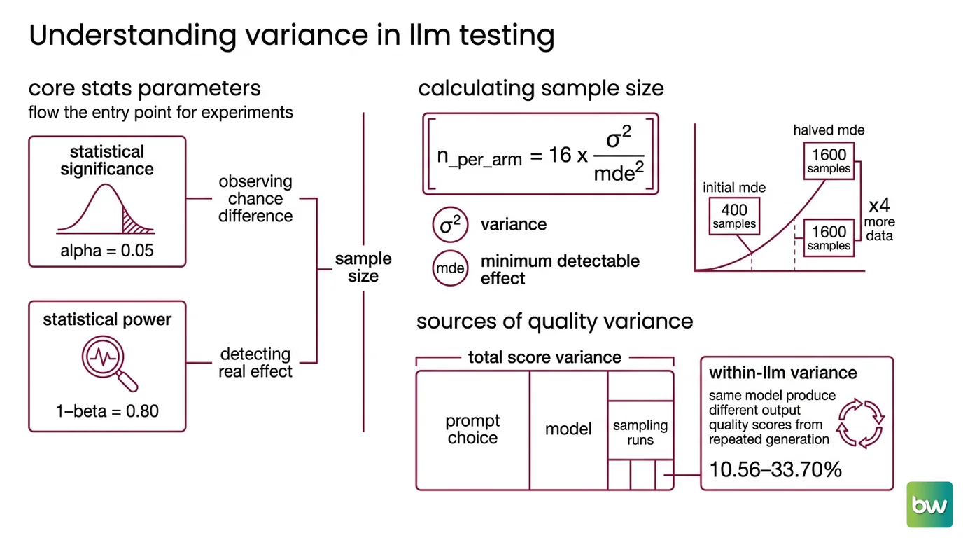
Statistical significance is the entry point. A result is significant at α = 0.05 when the probability of observing that difference by chance — assuming no real effect — falls below 5% (Cameron Wolfe, Deep Learning Focus). Statistical power (1 − β = 0.80) is the paired guarantee: an 80% chance of detecting a real effect when one actually exists. Together, these two parameters determine how large your experiment must be before any data is collected.

The sample size calculation for a two-arm experiment at these standard thresholds reduces to a useful approximation:

n_per_arm = 16 × σ² / MDE²

Where σ² is the variance of your quality metric and MDE is the minimum detectable effect — the smallest quality improvement you actually care about detecting (Cameron Wolfe, Deep Learning Focus). The relationship between MDE and sample size is quadratic, not linear: halving the MDE requires four times as many observations. If you want to detect a 2-point improvement on a quality rubric instead of a 4-point improvement, you need four times the data. This is not a rounding issue; it’s the mathematical structure of power analysis, and it bites teams that set their quality bar after the experiment has started.

The σ² term is where LLM evaluation departs from web analytics. Research on creative writing tasks decomposed total quality variance across models, prompts, and repeated sampling runs. Within-LLM variance — the same model producing different output quality scores across repeated generation — accounts for 10.56–33.70% of total score variance (arxiv 2601.21339). Prompt choice alone explains roughly 36.43% of quality variance, nearly matching model choice at 40.94% (arxiv 2601.21339). For creative tasks specifically, your experimental design is absorbing signal from both sources simultaneously.

Prompt variance rivals model variance.

The practical consequence is harder to dismiss than it looks. If you’re comparing Model A to Model B but you haven’t fixed — or at minimum controlled and balanced — the prompt across both arms, a substantial fraction of your measured difference reflects prompt sensitivity, not model quality. Your confidence interval is measuring a confound you didn’t know was present.

For the Central Limit Theorem to hold reliably on sample mean quality scores, you need at least n ≥ 100 observations per arm (Cameron Wolfe, Deep Learning Focus). Below that threshold, the normal approximation for mean quality scores degrades. Switch to bootstrapped confidence intervals: repeat sampling from your observed data to construct an empirical distribution of the mean difference, and check whether zero falls inside or outside the 95% interval.

Two Evaluation Modes, Two Different Questions

Two fundamentally distinct modes of LLM evaluation exist. They’re often treated as interchangeable because both produce quality metrics. They don’t answer the same question, and choosing the wrong one for your current uncertainty wastes experiment time.

Is online A/B testing on live traffic or offline dataset evaluation better for measuring LLM quality?

Offline evaluation uses a curated, fixed dataset. Both model variants run against identical inputs; outputs are scored and compared. Smaller datasets enable rapid iteration; larger datasets provide broader performance coverage (Label Studio). The signal is analytically clean — no user behavior noise, no traffic distribution shifts, no production serving latency introducing confounds. The limitation is the gap between your curated dataset and the actual distribution of queries users send to your system, which tends to widen over time.

Online A/B testing routes real traffic through Traffic Splitting to expose different user segments to different model variants. This captures behavioral signals that no dataset can simulate: re-query rates when an answer was unsatisfying, session abandonment when quality degraded, downstream task completion rates that reflect whether the model output actually helped. It also demands infrastructure that most teams underestimate at the planning stage. You need LLM Observability tooling to measure quality at serving time, Prompt Logging to capture request inputs for retrospective scoring, Distributed Tracing via OpenTelemetry to correlate quality signals across service boundaries, and careful Token Budget management to keep comparison arms cost-equivalent throughout the experiment window.

Offline catches regressions; online measures behavioral readiness.

Shadow Testing sits between these modes. The candidate model receives production-realistic traffic, but its outputs are never shown to users — you accumulate inputs that reflect real query distribution without exposing users to a potentially worse experience. The cost is inference on doubled traffic; the benefit is production-realistic inputs without behavioral risk. The gap is that user response signals remain unavailable — you still don’t know whether users would have found those outputs useful.

The practical sequence that reduces wasted live-traffic experiment budget: offline evaluation first to surface regressions on a curated holdout set, then shadow testing to validate behavior on production-realistic inputs, then live A/B testing only when the candidate has already cleared regression checks and you specifically need behavioral signal.

What the Variance Math Predicts in Production

Understanding the mechanism makes the failure modes predictable. LLM quality variance doesn’t only complicate sample size calculations — it creates specific, reproducible ways that otherwise well-designed experiments return misleading results.

What are the technical limitations of A/B testing for LLMs in production?

The first structural problem is independence. Standard t-tests assume observations are independent. LLM evaluation sets violate this routinely: if you sample 100 questions from the same domain corpus, the model’s responses are correlated — questions about the same topic elicit similar reasoning patterns, similar failure modes, and similar edge-case behaviors. This correlation inflates standard errors by up to 3× (Cameron Wolfe, Deep Learning Focus), widening your confidence intervals and making genuine quality differences statistically invisible even when sample counts look adequate on paper.

The second is distributional shape. LLM quality scores from rubric-based or LLM-as-judge evaluation pipelines rarely follow a Gaussian distribution. They cluster at score boundaries, show ceiling effects on simple tasks, and develop long tails on adversarial inputs. The sample size formula n = 16σ²/MDE² assumes normality; when your score distribution violates that assumption, the calculated sample size is wrong in ways that aren’t obvious from the formula alone. Bootstrapped 95% confidence intervals are the correction: resample from your observed data repeatedly, construct the empirical distribution of the mean difference, and check whether zero falls inside or outside that interval (Cameron Wolfe, Deep Learning Focus). For n < 100 or clustered data, bootstrapping should be the default method, not a fallback when parametric tests fail.

A practical variance reduction technique: generate K outputs per question rather than a single output, then average the scores. This reduces within-question variance by a factor of K (Cameron Wolfe, Deep Learning Focus). The cost scales linearly — K× the inference expense — making LLM Cost Management a constraint rather than an afterthought. Model Registry discipline becomes essential at this point: every evaluation data point needs its model version, temperature, and sample count recorded so that results are reproducible and comparable across experimental runs over time.

Reproducibility has a numerical target worth knowing. Running an evaluation pipeline ten times on identical data with randomness controlled should produce a coefficient of variation below 0.05 (arxiv 2506.13023). Above that threshold, measurement noise in your evaluation infrastructure begins to exceed the effect sizes most teams care about detecting. A CV above 0.05 means two runs of the same experiment on the same data can disagree — and you can’t distinguish real model differences from pipeline noise.

The evaluation tooling ecosystem introduces its own compatibility surface. As of mid-2026, Arize Phoenix released v8.0 with a major instrumentation overhaul; integrations built against v7.x may require updates. LangSmith’s Annotation Queues v2 replaced v1 with changed workflow APIs. RAGAS v0.2.x changed RAG metric APIs from v0.1.x, adding multi-turn evaluation but breaking backward compatibility. Treat eval tool upgrades as their own experimental comparison problem — pin specific versions and verify that metric values are stable across the transition before using cross-version results as baselines.

Compatibility note:

• Arize Phoenix v8.0: Major UI and instrumentation overhaul; v7.x integrations may need updates (Inference.net).
• LangSmith Annotation Queues v2: Replaced v1 — older workflow integrations may break (Inference.net).
• RAGAS v0.2.x: Multi-turn metrics added; RAG metric APIs changed from v0.1.x (Inference.net).

Clustering kills your standard errors. When you cannot guarantee independence across your evaluation set — which is most of the time in practice — design for it explicitly: stratify your sampling across topic clusters, use cluster-robust standard error estimators, or default to bootstrapping.

Rule of thumb: Before comparing two models, measure the within-model variance of each using repeated sampling on a fixed holdout set. If either model’s internal variance exceeds the quality difference you want to detect, no experiment will resolve the question without substantially more observations than your initial calculation suggested.

When it breaks: The entire A/B testing framework assumes a stable measurement instrument. If your judge model, scoring rubric, or evaluation prompt changes between experimental arms — or between the baseline measurement and the comparison measurement — you’re measuring evaluation pipeline variance rather than model quality. Results that cross this boundary are not A/B tests; they produce numbers that look like evidence and mean nothing.

The Data Says

Within-LLM variance absorbs 10.56–33.70% of total quality score variance for creative tasks, and prompt choice explains another ~36% — nearly as much as model choice itself. The sample size math is clean, but the quadratic relationship between minimum detectable effect and required observations means small experiments systematically fail to resolve the quality differences that actually matter in production. Valid LLM A/B testing is not harder than web testing because the statistics are different; it’s harder because the variance is higher, its sources are more entangled, and the measurement instrument itself requires versioning.