Class Imbalance Prerequisites: Confusion Matrices, PR-AUC, Data-Level vs Algorithm-Level
ELI5
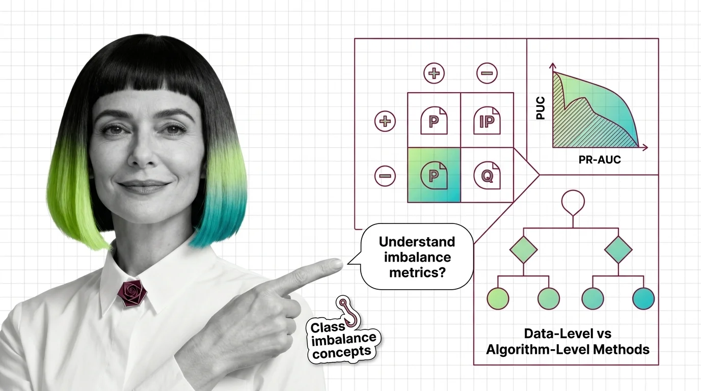
Class imbalance is when one outcome is rare — fraud, disease, defects. Before fixing it, you need three things: a confusion matrix to see the errors, metrics that ignore the majority, and a choice between reshaping data or reweighting the model.
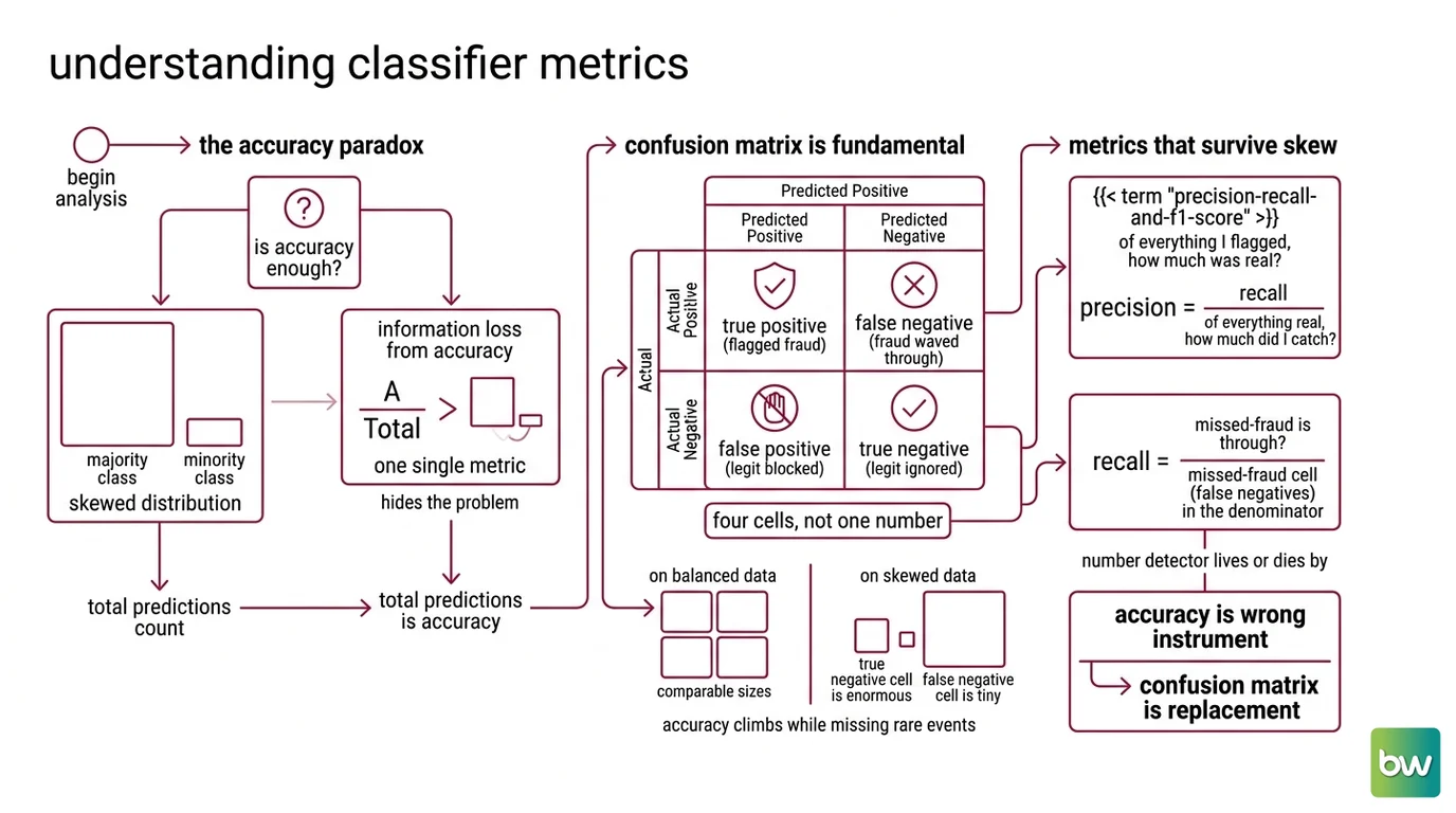
A fraud model can be right 999 times out of 1,000 and still be useless. If real fraud appears in about one transaction per thousand, a model that labels everything “legitimate” scores 99.9% accuracy and catches zero fraud. The dashboard looks excellent; the system is worthless. That gap between a flattering metric and a failing model is where every Class Imbalance problem begins.
The Matrix Underneath Every Classifier
The accuracy paradox is not a flaw in the metric. Accuracy faithfully reports the fraction of correct predictions; it simply turns out that on a skewed distribution, being right about the boring majority swamps being wrong about the rare event you actually care about. To see the error, you have to stop counting totals and start counting kinds of error.
What do you need to understand before learning class imbalance techniques?
Before any resampling trick or weighted loss, one object sits beneath everything else: the Confusion Matrix. It splits predictions into four cells — true positives, false negatives, false positives, and true negatives. A true positive is fraud the model flagged. A false negative is fraud it waved through. A false positive is a legitimate charge it blocked. A true negative is a clean charge it correctly ignored.
Accuracy collapses these four numbers into one ratio, and that collapse is exactly the information loss that hides the problem. On a balanced dataset the four cells are roughly comparable, so the single number behaves. On a skewed one, the true-negative cell is enormous and the cell you care about — the false negatives — is tiny, so a model can grow that big cell, shrink nothing useful, and watch its accuracy climb.
Not one number. Four.
From those four cells come the two ratios that matter under skew. Precision, Recall, and F1 Score reframes the question: precision asks “of everything I flagged, how much was real?” while recall asks “of everything real, how much did I catch?” The missed-fraud cell — the false negatives — sits in the denominator of recall, which is why recall is usually the number a rare-event detector lives or dies by. The lesson before you touch a single technique: accuracy is the wrong instrument for a rare event, and the confusion matrix is the one you replace it with.
Metrics That Survive a Skewed Distribution
Once accuracy is off the table, you need summary numbers that stay honest when one class dominates. The trap is that some popular metrics look rigorous while quietly inheriting the same blind spot as accuracy.
Which evaluation metrics should you know for imbalanced classification?
Start with the precision-recall curve. As you sweep the classification threshold from strict to permissive, precision and recall trade against each other, and the curve traces that trade-off for the minority class specifically. To compress it into one number, scikit-learn’s average_precision_score takes a weighted mean of the precisions at each threshold, weighted by the gain in recall — deliberately not the trapezoidal area under the curve, which interpolates between points too optimistically (scikit-learn docs). When people say “PR-AUC,” the concrete, defensible function is average_precision_score, and the distinction matters because the interpolated version can quietly inflate a weak model.
Contrast this with Roc Auc, the metric most teams reach for by reflex. The ROC curve plots recall against the false-positive rate, and the false-positive rate divides by the count of true negatives. Under heavy imbalance that count is gigantic, so even a flood of false positives barely nudges the axis. The result: ROC-AUC flatters an imbalanced model, reporting a strong score while precision stays poor. The precision-recall view does not offer that comfort, which is precisely why it is the more truthful summary here.
For a single threshold-aware number, balanced_accuracy_score averages recall across the classes rather than across the samples (scikit-learn docs). It is the macro-average of per-class recall, so the rare class gets equal weight to the common one — the minority can no longer be ignored into a good score. Three numbers, then, before you change anything about the model: average precision for the curve, recall for the cost of misses, and
Balanced Accuracy for a fair single figure.
Two Families, Two Philosophies
Only now — after the matrix and the metrics — do the actual remedies make sense. Every technique for class imbalance belongs to one of two families, and the split is clean: you can change the data the model sees, or you can change the rule by which it learns.
What is the difference between data-level and algorithm-level methods for class imbalance?
Data-level methods rebalance the training distribution before the model ever sees it. The blunt versions are Oversampling, which duplicates minority examples, and Undersampling, which drops majority ones. The refined versions synthesize new minority points instead of copying them: SMOTE, introduced by Chawla and colleagues in 2002 (JAIR), interpolates between a minority example and its nearest minority neighbors to invent plausible new cases. ADASYN, from He and colleagues in 2008 (IEEE IJCNN 2008), pushes that idea further by generating more synthetic samples for the minority points that sit in hard, majority-dominated regions — concentrating effort where the boundary is most contested.
Algorithm-level methods leave the data untouched and rewrite the objective.
Class Weighting tells the model that an error on the rare class costs more, and in scikit-learn class_weight='balanced' sets those weights inversely proportional to class frequency (scikit-learn docs).
Cost Sensitive Learning generalizes this to a full cost structure, where each kind of mistake carries its own price.
Focal Loss reshapes the loss itself to down-weight easy, already-correct examples so training focuses on the hard minority cases — though it came from object detection, not tabular data, where Lin and colleagues introduced it in 2017 for the RetinaNet detector (Lin et al., RetinaNet). Treat it as a loss-reweighting idea to adapt, not a drop-in function.
The dividing line is simple enough to keep in your head: data-level changes the data; algorithm-level changes the objective.
| Family | What it changes | Examples | Main risk |
|---|---|---|---|
| Data-level | The training distribution | Random oversampling, random undersampling, SMOTE, ADASYN | Leakage if applied before splitting; undersampling discards real signal |
| Algorithm-level | The learning objective | class_weight='balanced', cost-sensitive learning, focal loss | Needs estimator support; weights must reflect real error costs |
As of mid-2026, the standard scikit-learn-contrib library for the data-level family is Imbalanced Learn 0.14.2, which implements SMOTE, ADASYN, and the random samplers, and which requires scikit-learn 1.5 or newer (imbalanced-learn docs).
Where Resampling Quietly Leaks
Understanding the two families is half the battle. The other half is knowing the one mistake that silently destroys every honest metric you just learned to compute — and it hides inside the data-level family.
Synthetic samples are built from real ones. If you run SMOTE on the full dataset and then split into training and validation folds, synthetic points generated from a real sample can land in the training fold while their parent lands in validation. The model has effectively seen the answer key. This is textbook Data Leakage, and it inflates your scores in a way that survives every check until production exposes it. The hard rule: resample only inside each fold of Cross Validation, fitting the sampler on the training portion alone. In practice, that means wrapping the sampler and estimator in a pipeline so the resampling step refits per fold.
That single discipline turns understanding into prediction:
- If you resample before splitting, your cross-validation scores will look strong and production will disappoint — that gap is the leak.
- If ROC-AUC looks excellent but precision is weak, the model is exploiting the majority class; trust the precision-recall view instead.
- If undersampling lifts validation scores but the model misses rare sub-types, you discarded majority examples that carried the decision boundary.
Rule of thumb: Pick the metric before the method. If a missed positive costs far more than a false alarm, optimize recall, report average precision, and then choose the rebalancing technique that actually moves those numbers — not the one that is most fashionable.
When it breaks: Synthetic oversampling assumes the minority class is locally continuous — that a point sitting between two fraud cases is also fraud. When the minority is multi-modal or the features are categorical, SMOTE invents samples in empty regions of the real distribution, and the model learns to trust a fiction.
The Data Says
Class imbalance is not solved by a single function call; it is solved by reading the confusion matrix, choosing metrics that refuse to be fooled by the majority, and then picking a remedy from the right family. Average precision and balanced accuracy tell you whether the rare class is actually being caught, while ROC-AUC will reassure you even when it is not. Get the leakage rule wrong and none of the rest counts.
AI-assisted content, human-reviewed. Images AI-generated. Editorial Standards · Our Editors