Pre-Filter vs Post-Filter vs Filtered-HNSW: Metadata Filtering at Scale
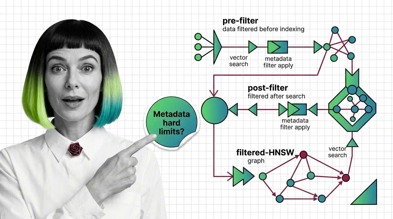
Table of Contents
ELI5
Metadata filtering narrows a vector search to records matching attribute predicates. It looks like a SQL WHERE clause on similarity search. It is not. The graph that makes vector search fast collapses when filters get strict, and recall drops silently.
A team ships a clean little function. They take a
Metadata Filtering predicate — tenant_id = 'acme' AND created_at > '2026-01-01' AND doc_type IN ('contract','memo') — pass it to their vector store, and assume the engine handles the rest. The query returns ten neighbors. The latency looks fine. The eval set looks fine. Three months later, a regulated customer finds a document that the system “knew about” but never surfaced for a query it should have answered. No exception fired. No log line complained. The recall just quietly went sideways for a particular slice of the data, on a particular shape of filter, and nobody saw it because the API kept returning ten results.
The wrong mental model is that a filter is a WHERE clause and the vector search is the ORDER BY. Two independent operations, composable in either order. That model is exactly what generates the bug above. The reality is geometric: the filter changes the graph the search is allowed to walk on, and the navigability of that graph is what determines whether the result set is a true approximation of the nearest neighbors or a polite lie.
The Three Strategies Hiding Behind One API Call
Every vector store with metadata support — Qdrant, Weaviate, Milvus, pgvector, Pinecone — implements one of three filtering strategies, sometimes more than one, and switches between them by heuristic. The user-visible API is identical. The behavior under load is not. Before you can debug filtered search, you have to know which mode you are actually in, and that requires three pieces of background knowledge.
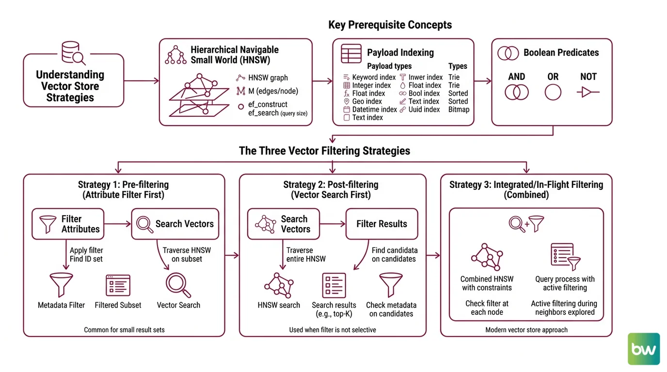
What concepts do you need to understand before metadata filtering: HNSW, payload indexing, and Boolean predicates?
The first prerequisite is the index that makes vector search fast in the first place. Almost every modern vector store builds on HNSW — Hierarchical Navigable Small World graphs, introduced by Malkov and Yashunin in 2016 (the Malkov & Yashunin paper). HNSW arranges vectors as a layered graph where higher layers contain a sparse subset of nodes connected by long-range edges, and lower layers contain everything connected by shorter, denser edges. Three parameters define its character: M, the number of edges per node — Qdrant defaults to 16; ef_construct, the number of neighbors considered while building — default 100; and ef (or ef_search), the candidate list size at query time — pgvector defaults to 40 (Qdrant Docs). A query starts at the top layer, greedily walks toward the query vector, then descends. The whole thing works because the graph has the small-world property: most nodes are reachable from most other nodes in a logarithmic number of hops.
The second prerequisite is the payload index. Vector stores index attributes the same way relational databases do, but with a typology shaped by the predicate kinds you actually want to push down. Qdrant supports keyword, integer, float, bool (since v1.4), geo, datetime (v1.8+), text, and uuid (v1.11+) payload indexes (Qdrant Docs). Milvus splits scalar indexes into Trie for VARCHAR, sorted indexes for numerics, Bitmap for low-cardinality tags accessed via in or array_contains, and an Inverted Index for text matching (Milvus Docs). The choice of index type determines whether a predicate can be evaluated as a fast set lookup or whether the engine has to fall back to a full scan.
The third prerequisite is the Boolean predicate language itself. Filters are expressions over indexed fields with AND, OR, NOT, range operators, and set membership. The relevant property is not their syntax but their selectivity — the fraction of the corpus they admit. A predicate that matches one percent of documents behaves nothing like one that matches ninety percent, even if the SQL looks similar.
These three concepts collapse into a single question the query planner has to answer at every call: given this predicate, can I walk the HNSW graph and expect to find good neighbors, or should I evaluate the predicate first and search only the survivors?
Pre-filter, post-filter, filtered-HNSW: where each strategy lives
Post-filtering is the naive baseline. Run the ANN search, return the top k * f candidates, then drop the ones that fail the predicate. It is correct when the filter has high selectivity (matches most documents) and catastrophic when it does not. If your filter admits one percent of the corpus and you ask for ten neighbors, you might need to over-fetch a thousand candidates to expect any survivors, and even then you are scanning the wrong neighborhood of the graph.
Pre-filtering is the conceptually clean alternative. Evaluate the predicate first, get a set of allowed IDs, and run vector search restricted to that set. Milvus is structured this way by design — filtering is always pre-filtering, with the scalar predicate evaluated first and ANN search ignoring rejected rows (Milvus Docs). The trap is that “search restricted to that set” is doing real work: if the allowed set is small, you can brute-force it and recall is perfect; if the allowed set is large but disconnected from the dense regions of the HNSW graph, you may end up scanning more than you would have without the filter.
Filtered-HNSW is the recent answer to that trap. Instead of evaluating the predicate around the graph, the predicate becomes part of how the graph is walked. Qdrant calls its variant Filterable HNSW — it extends the standard graph with extra edges based on indexed payload values, and a query planner picks between HNSW traversal and a payload-index full scan based on estimated cardinality (Qdrant Docs). Below the full_scan_threshold (default 10,000 KB of estimated filtered subset), Qdrant abandons graph traversal and rescores via the payload index. Weaviate’s default since v1.34 is ACORN, a multi-hop strategy from Patel et al. that performs predicate-agnostic graph construction and uses 2-hop neighbor expansion at query time to keep the predicate subgraph connected when filters remove nodes and edges (the ACORN paper). Weaviate also automatically switches to brute-force flat search around a 15% match-rate threshold (Weaviate Docs).
The strategies are not interchangeable. They are different bets about what the filter looks like.
Where the Math Stops Cooperating
Filtering is not free, and the cost is not paid in latency — it is paid in recall, and recall failures are silent. The interesting failures come from a small number of mechanisms that compound at scale.
What are the technical limits of metadata filtering: recall collapse, cardinality explosion, and filter selectivity trade-offs?
Recall collapse is the failure mode that gives this section its name. HNSW works because the graph has the small-world property — short paths between most pairs of nodes, supported by long-range edges in the upper layers. A filter that removes nodes and the edges incident to them does not remove the surviving graph’s nodes; it removes the property that makes the graph navigable. When most nodes or edges are filtered out, the predicate subgraph fragments into disconnected components, and the search converges on whichever component the entry point happens to land in (the ACORN paper). Recall does not degrade smoothly — it falls off a cliff at a selectivity threshold that depends on the graph’s M, the original ef parameters, and the spatial correlation between the filter and the query.
ACORN’s 2-hop neighbor expansion mitigates this — when an edge points to a filtered-out node, the search “sees through” it to that node’s neighbors, restoring connectivity. The original benchmarks reported 2-1000× throughput improvements at fixed recall over prior filtered-ANN methods (the ACORN paper), though the range is dataset-dependent and the upper end reflects best-case selectivity profiles. On extremely sparse subgraphs, even ACORN-style expansion still degrades.
Cardinality explosion is the failure mode of the query planner, not the index. Filterable-HNSW systems estimate the size of the filtered subset before they commit to a strategy: high estimated cardinality (a permissive filter) means walk the HNSW graph; low estimated cardinality (a restrictive filter, small allowed set) means rescore via the payload index full scan (Qdrant Docs). When the estimate is wrong — bad statistics, skewed distributions, correlated predicates — the planner picks the wrong strategy and you pay either a brute-force scan you didn’t budget for or a graph walk that converges on the wrong region. The bug is hard to reproduce because it depends on the query mix, the data distribution at that moment, and the planner’s hysteresis around its threshold.
Filter selectivity trade-offs are the broader principle. There is a sweet spot where the filter is selective enough to matter and permissive enough that the surviving subgraph still has small-world properties. Outside that band, every strategy has a regime where it fails: post-filter at low selectivity, pre-filter at large allowed sets that are spatially disjoint from the query, filtered-HNSW at extreme sparsity. The system that gives you “filtering, just specify the predicate” is hiding a planner that is making a guess on every call.
Implementation notes:
- pgvector pre-0.8.0: versions before 0.8.0 silently return under-filled result sets when a
WHEREfilter reduces candidates below the requestedk— the canonical post-filter recall failure. Fix: upgrade to 0.8.0+ and enablehnsw.iterative_scaninstrict_orderorrelaxed_ordermode (default off;hnsw.max_scan_tuplesdefaults to 20,000) (pgvector’s GitHub repository).- Weaviate v1.34+: ACORN is the default
filterStrategyon the HNSW vector index; older configs may still default tosweeping. Verify the strategy explicitly in the schema if you migrated from an earlier version (Weaviate Docs).- Milvus 2.5+: Bitmap and Inverted-Index Text Match are new in 2.5 and improve filtered-search throughput on text and tag fields versus 2.4’s wildcard match (Milvus Docs). Enable them on fields you actually filter on; they are not automatic.
What the Geometry Predicts
The mechanism turns the filtered-search bug into something you can reason about before you hit it.
If your filter is highly permissive (excluding very little of the corpus), all three strategies converge to roughly the same recall, and you should optimize for latency. As selectivity tightens into a middle band where the surviving subgraph still has small-world properties, filtered-HNSW with cardinality-aware planning is doing real work for you, and the choice of database matters. At extreme selectivity — when only a small fraction of the corpus survives — you are in brute-force territory regardless of what the API call looks like: Weaviate flips to flat search around a 15% match-rate threshold, and Qdrant abandons graph traversal for a payload-index scan below full_scan_threshold (Weaviate Docs, Qdrant Docs). The exact crossover points are dataset-dependent — measure them on your own data rather than trusting fixed percentages.
If you change M or ef_search, expect recall to move non-monotonically when filters are present. Higher M adds robustness against filter-induced fragmentation; higher ef_search increases the candidate list and helps the search escape disconnected components — both at a latency cost.
If you correlate your filter with your query (for example, filtering on topic = 'finance' while querying with a finance-shaped vector), the surviving subgraph stays dense in the relevant region and recall holds. If you anti-correlate them (filtering on topic = 'sports' while querying with a finance vector), the subgraph the search has to walk is the sparse, distant part of the index, and recall falls fastest there.
Rule of thumb: Measure recall at the actual filter selectivity profile your production traffic has, not at uniform random. The recall-vs-selectivity curve is the diagnostic.
When it breaks: Filtered-HNSW recall collapses sharply when filter selectivity drives the predicate subgraph below the small-world connectivity threshold, and the failure is silent — the API still returns k results, just from the wrong neighborhood of the graph.
The Hidden Assumption Underneath All of This
Every filtering strategy assumes the predicate is independent of the embedding geometry. That assumption almost never holds. Filters are usually correlated with the same semantic structure the embeddings encode — language = 'de' co-occurs with German-shaped vectors; tenant_id = 'acme' co-occurs with whatever Acme writes about. When the correlation is strong and aligned with the query, filtering helps; when it is strong and orthogonal to the query, filtering destroys the navigability the index was designed around. The hardest filtered-search bugs are the ones where the predicate is doing two jobs at once — narrowing the result set and reshaping the latent space — and only one of those jobs is visible in the query plan.
This is also why filtered vector search is not a substitute for Knowledge Graphs For RAG when the retrieval task has structural relationships the embedding geometry never encoded — predicate-augmented HNSW reshapes a similarity space, it does not introduce one. And the metadata fields you are filtering on have to come from somewhere upstream: weak Document Parsing And Extraction produces sparse, inconsistent payloads, and the planner’s cardinality estimates are only as honest as the index it is reading.
The Data Says
Metadata filtering is not a WHERE clause; it is a deformation of the index’s navigability, evaluated by a planner that is guessing about your data. The strategies — post-filter, pre-filter, filtered-HNSW — are different bets about how that deformation behaves, and every modern vector store hides which bet it is making behind a uniform API. Know your filter selectivity profile, know which strategy your database picks at each selectivity band, and measure recall at the predicates your production actually runs.
AI-assisted content, human-reviewed. Images AI-generated. Editorial Standards · Our Editors