Memory Blowup, Recall Collapse, and the Hard Engineering Limits of Vector Indexing at Scale
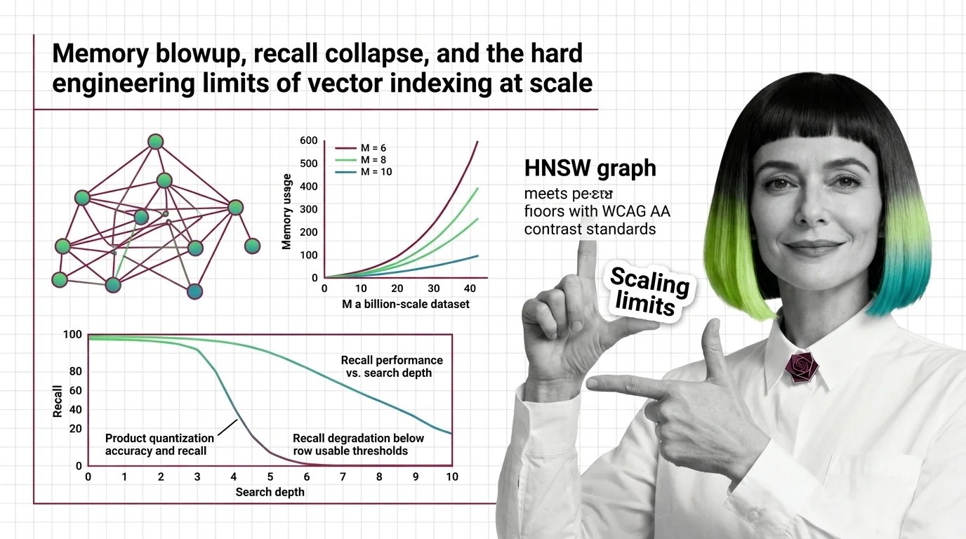
Table of Contents
ELI5
Vector indexing trades memory for search speed, but at billion-scale these trades turn brutal — memory grows linearly with graph connectivity while compression destroys the accuracy you built the index to preserve.
Here is an observation that should bother you: the same algorithm that retrieves your nearest neighbors in milliseconds on ten million vectors will demand over a terabyte of RAM at a billion. The math did not change. The engineering constraints just stopped being polite. Most teams discover this after they have committed to an architecture, and by then, the options are expensive.
The Graph That Memorizes Everything — and the Cost of Its Memory
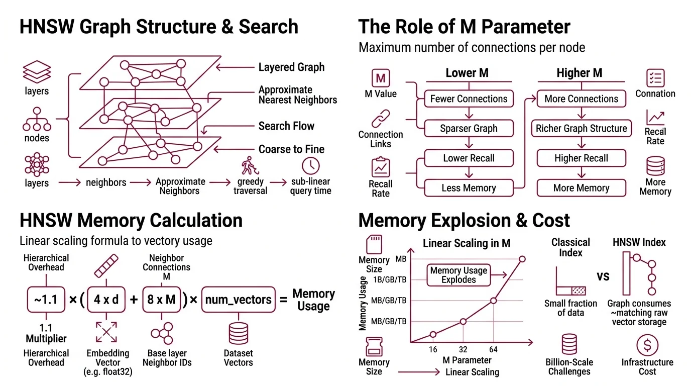
Vector Indexing at scale is dominated by one data structure: the Hierarchical Navigable Small World graph. Introduced by Malkov & Yashunin in 2016, HNSW builds a layered graph where each node connects to its approximate nearest neighbors, and search proceeds by greedy traversal from coarse upper layers to fine lower layers. The elegance is real — HNSW delivers sub-linear query time with high recall. But that elegance has a price measured in bytes per connection, and the invoice arrives at scale.
Why does HNSW memory usage explode with high M values and billion-scale datasets?
The parameter M controls how many neighbors each node maintains. Higher M means more connections, richer graph structure, better recall during traversal. It also means the index becomes a memory furnace.
The formula is not subtle:
~1.1 x (4 x d + 8 x M) x num_vectors bytes
Each node stores its Embedding vector (4 bytes per dimension for float32) plus 2*M neighbor IDs at the base layer (Lantern Blog). The 1.1 multiplier accounts for upper-layer overhead in the hierarchical structure.
Run the arithmetic on a concrete case. One billion vectors at 128 dimensions with M=16 — a moderate connectivity setting — requires approximately 1,408 GB of memory including replication (Lantern Blog). That is not a provisioning problem. That is a different category of infrastructure.
The scaling is linear in M. Double the connectivity parameter, double the graph memory. On Sift1M with M=64, the graph structure alone consumes roughly 512 MB — matching the raw vector storage — pushing total memory to approximately 1 GB for just one million vectors (Weaviate Blog). The graph becomes as expensive to store as the data it indexes.
This is where the intuition breaks. In classical databases, the index is a small fraction of the data. In HNSW, the index IS the data — and then some. The vectors themselves are only half the memory cost; the other half is the graph topology your queries traverse.
The implication is architectural: you cannot solve billion-scale HNSW by adding RAM. Or rather, you can, but the cost curve bends upward fast enough to reframe whether vector search was the right abstraction in the first place.
Compression as a Wager — What You Lose When You Quantize
Memory is the wall. The standard response is compression: reduce each vector’s footprint by approximating it. Product Quantization is the most widely used technique, originating from Jegou, Douze, and Schmid’s 2011 IEEE TPAMI paper. The core idea is elegant in the way all lossy compression is elegant — it works until the geometry disagrees.
PQ splits each high-dimensional vector into subspaces — a 128-dimensional vector might become 16 subspaces of 8 dimensions each — then replaces each subspace with the ID of its nearest centroid from a learned codebook. Instead of storing the full vector, you store a short code: a sequence of centroid indices. Memory drops dramatically. On 1 million Sphere vectors, PQ achieved an 85-90% reduction, compressing 5 GB to 725 MB (Weaviate Blog).
The cost is accuracy. And the cost is not uniform.
How much accuracy does product quantization lose and when does recall degrade below usable thresholds?
The answer depends on where your data lives in the geometry of the Similarity Search Algorithms space — and this is where the engineering gets precarious.
On well-behaved datasets like Sift1M (128-dimensional, cleanly clustered), PQ recall drops are modest: 0.2-0.3 percentage points under moderate compression. A system achieving 0.9997 recall uncompressed might drop to 0.9966 compressed (Weaviate Blog). Barely perceptible.
On harder datasets, the story shifts. On Gist (960-dimensional, less structure), recall drops 1.1-4.2 percentage points — from 0.996 down to 0.955 at high parameter settings (Weaviate Blog). Still functional, but the gap is widening with every added dimension.
Now push further. Take 1536-dimensional embeddings — the kind produced by modern transformer models — and apply aggressive PQ. In one Weaviate benchmark, Recall@10 collapsed below 10% compared to exact search (Weaviate Blog). The figure comes from a single test; other implementations may behave differently. But the direction is unmistakable: at high dimensionality, aggressive quantization can destroy the structure it was meant to compress.
Not compression. Destruction.
The mechanism behind this collapse is geometric. PQ assumes that variance distributes roughly evenly across subspaces. When it does not — when certain dimensions carry disproportionate information, as they often do in high-dimensional transformer embeddings — the codebook approximation shatters. The centroids in each subspace no longer capture the meaningful structure of the original vectors; they capture an average that represents nothing.
At billion scale, though, compression is not optional. A billion 1536-dimensional vectors uncompressed would exceed 5 TB. PQ can bring that to roughly 0.7 TB from 2.7 TB on the Sphere billion-vector dataset, approximately 74% reduction (Weaviate Blog). The memory savings are real. The question is whether the recall you surrender makes the system usable or merely cheaper.
PQ rescoring can nearly eliminate the recall gap — reranking compressed results against original vectors stored on disk. Weaviate introduced this in v1.21 (Weaviate Blog). But rescoring adds latency, and at billion scale, that latency compounds across every query.
The Responses — Disk, Redundancy, and Newer Compression
The engineering community’s response to these constraints splits along a predictable fault line.
DiskANN takes the disk-based path. Developed at Microsoft (Subramanya et al., NeurIPS 2019), it stores the graph on SSD rather than RAM, using a Vamana graph structure designed for sequential disk reads. On one billion SIFT vectors, DiskANN achieves over 5,000 queries per second at sub-3ms latency with 95%+ recall on a single node with 64 GB RAM plus SSD (Microsoft Research). The trade is latency variance; SSD access patterns are less predictable than RAM, and tail latencies widen under concurrent load.
ScaNN takes a different angle. Its SOAR algorithm introduces controlled redundancy through multi-cluster assignment — vectors belong to more than one IVF (Inverted File Index) partition, sacrificing memory for faster search with smaller indexes (Google Research Blog). Google’s Vertex AI Vector Search 2.0, built on ScaNN, reports approximately 99% ANN accuracy at sub-10ms latency at billions of vectors (Google Cloud Docs).
Faiss, Meta’s library, remains the most widely deployed implementation for both HNSW and IVF-PQ. Its v1.14.0 release introduced RaBitQ — a binary quantization method that offers an alternative compression path to PQ — and Dynamic Dispatch for architecture-specific optimization, with the current version at v1.14.1 (March 2026) (FAISS GitHub).
The recall gap between fundamental approaches is stark. On a 100-million-vector benchmark, HNSW achieved approximately 0.87 recall while IVF-PQ reached approximately 0.61 (Weaviate Blog). Twenty-six percentage points of missed results — the price of compression, measured in answers your users never see.
Compatibility note:
- DiskANN: Major Rust rewrite in progress (v0.49.1, March 2026). The C++ codebase has moved to the
cpp_mainbranch and is no longer actively maintained. Evaluate language stability before production adoption (DiskANN GitHub).
Where the Engineering Envelope Tears
The practical consequence of these limits is that billion-scale vector search forces a three-way trade-off: memory, recall, and latency. You get two.
High recall and low latency costs memory — HNSW with high M on large RAM instances. Low memory and acceptable recall costs latency — PQ with rescoring, or DiskANN with SSD. Low memory and low latency costs recall — aggressive PQ without rescoring, and your application had better tolerate returning wrong neighbors some fraction of the time.
If you change the dimensionality of your embeddings, expect the compression trade-off to shift non-linearly. A model upgrade from 768-d to 1536-d does not double your PQ recall loss — it can multiply it by an order of magnitude, because the geometric assumptions PQ relies on grow more fragile with every added dimension. If you increase M to recover recall, expect your memory bill to increase linearly with the parameter and linearly with your dataset size — no diminishing returns, no plateau.
Rule of thumb: On datasets with dimensionality above 768, benchmark PQ recall on YOUR data before committing to a compression ratio. Sift1M numbers transfer poorly to production embedding spaces.
When it breaks: The limits converge hardest at the intersection of high dimensionality (1536-d transformer embeddings) and aggressive memory pressure. In that regime, PQ recall can collapse catastrophically — and the standard mitigations (rescoring, higher nprobe) add precisely the latency you were trying to avoid. Billion-scale memory estimates also vary by 2-3x depending on replication factors and neighbor ID bit widths, making capacity planning more guess than calculation.
The Data Says
Vector indexing at scale is a sequence of trades, not solutions. HNSW memory scales linearly with connectivity and there is no algorithmic shortcut around it. PQ compression works until high dimensionality breaks its geometric assumptions — and modern embeddings break those assumptions routinely. The engineering discipline is not choosing the best algorithm; it is knowing which trade-off your application can survive.
AI-assisted content, human-reviewed. Images AI-generated. Editorial Standards · Our Editors