Inter-Annotator Agreement, Annotation Guidelines, and the Building Blocks of a Labeling Project
ELI5
Inter-annotator agreement measures whether two people labeling the same data actually agree — after subtracting the agreement you would expect from random guessing. High raw agreement can still hide labels that are barely better than chance.
Two annotators label the same batch of support tickets and agree on the overwhelming majority of them. The project lead calls it a win. Then someone runs the same labels through Cohen’s kappa and the score comes back near zero — sometimes negative. Nothing about the labels changed. Only the way we counted agreement did, and that single change exposes a dataset that was never as clean as it looked.
This is the uncomfortable opening fact of any labeling effort: the number that feels most reassuring — “they agreed almost every time” — is the one most likely to lie to you. Understanding why is the difference between a dataset you can train on and a pile of confident noise.
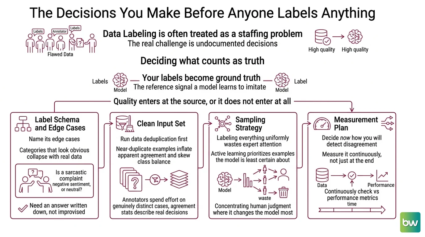
The Decisions You Make Before Anyone Labels Anything
Most teams treat Data Labeling And Annotation as a staffing problem — hire annotators, hand them data, collect labels. The expensive failures happen earlier, in the decisions nobody documents. A label schema is a measurement instrument, and an instrument with ambiguous units produces ambiguous readings no matter how careful the people holding it are.
What do you need to understand before starting a data labeling project?
Before a single example gets a label, you are really deciding what counts as truth. The labels you collect become your Ground Truth — the reference signal a model learns to imitate. If that reference is inconsistent, the model faithfully learns the inconsistency, and no amount of architecture or compute corrects for it. This is the central claim of Training Data Quality work: quality enters at the source, or it does not enter at all.
Four decisions deserve attention before labeling starts:
- A label schema that names its edge cases. Categories that look obvious in a planning meeting collapse the moment annotators meet real data. “Is a sarcastic complaint negative sentiment, or neutral?” needs an answer written down, not improvised per annotator.
- A clean input set. Near-duplicate examples inflate apparent agreement and skew class balance. Running Data Deduplication first means your annotators spend effort on genuinely distinct cases, and your agreement statistics describe real decisions rather than the same item counted twice.
- A sampling strategy. Labeling everything uniformly wastes the most expensive resource you have — expert attention. Techniques like Active Learning prioritize the examples the model is least certain about, concentrating human judgment where it changes the model most.
- A measurement plan. Decide now how you will detect disagreement, because you will measure it continuously, not at the end.
Skip these, and you do not find out until the model underperforms — by which point the cause is buried under thousands of labels. The cheapest moment to fix a labeling project is before it starts.
The Statistics of Agreeing by Accident
Here is where the reassuring numbers turn on you. Raw agreement — the percentage of items two annotators labeled identically — counts every match equally, including the matches that would have happened by luck. When one category dominates the data, luck does a lot of the work.
What is inter-annotator agreement and how is Cohen’s kappa calculated?
Inter Annotator Agreement asks a sharper question than “how often did they match?” It asks: how often did they match beyond what chance alone would produce? Cohen’s kappa, introduced by Jacob Cohen in 1960, formalizes this as a ratio. Its formula is compact:
κ = (pₒ − pₑ) / (1 − pₑ)
where pₒ is the observed agreement and pₑ is the agreement expected by chance, per Cohen (1960). The numerator strips out luck; the denominator scales the result against the best you could have done. The output runs from −1 to +1: a kappa of +1 means perfect agreement, 0 means agreement no better than chance, and a negative value means the annotators agreed less than random labeling would predict.
Work a small case to see the trap. Imagine two annotators sorting 100 messages into spam or not-spam. They agree on 90 of them, so pₒ is 0.90. But spam is rare here — each annotator flags only 5 messages as spam and calls the other 95 clean. The agreement you would expect from chance is the probability they both say spam plus the probability they both say clean: (0.05 × 0.05) + (0.95 × 0.95), which works out to 0.905. Drop those into the formula — (0.90 − 0.905) / (1 − 0.905) — and kappa lands at roughly −0.05.
Ninety percent agreement. A kappa below zero.
Not a calculation error. An emergent property of skewed data. When one label dominates, two annotators clicking the majority class out of habit will agree constantly, and kappa correctly reports that almost none of that agreement carries information. This is the prevalence effect, and it is exactly why raw agreement cannot be trusted as a quality signal on imbalanced datasets.
So how do you read a kappa once you have one? A commonly cited rule of thumb from Landis & Koch (1977) maps the scale like this: below 0.00 is poor, 0.00–0.20 slight, 0.21–0.40 fair, 0.41–0.60 moderate, 0.61–0.80 substantial, and 0.81–1.00 almost perfect. Treat it as convention, not law — Landis & Koch (1977) offered no empirical basis for those exact cutoffs, and what counts as “good” depends entirely on the task. Part-of-speech tagging routinely expects agreement above 0.80; subjective sentiment work may be healthy at far lower values.
Which agreement metric fits your annotation setup
Cohen’s kappa has a hard boundary: it compares exactly two annotators on nominal categories, per Cohen (1960). The moment your setup changes, the metric has to change with it — and assuming kappa scales to a team is a frequent, silent mistake.
| Your setup | Metric | Why |
|---|---|---|
| Exactly 2 annotators, nominal labels | Cohen’s kappa | The original two-rater, chance-corrected coefficient (Cohen, 1960) |
| 3+ fixed raters, every item labeled by all | Fleiss’ kappa | Generalizes Cohen’s κ to many interchangeable raters, aggregating agreement across the group rather than pairwise (Fleiss, 1971) |
| Variable raters per item, missing data, or ordinal/interval labels | Krippendorff’s alpha | The most flexible option — handles any number of raters, gaps, and non-nominal data, as documented by the Label Studio Blog |
The selection rule is mechanical once you state it plainly: two raters means Cohen’s kappa, three or more fixed raters means Fleiss’ kappa, and anything with variable raters, missing labels, or non-nominal data means Krippendorff’s alpha. Pick the metric that matches your data’s shape, not the one that returns the friendliest number.
The Machinery That Manufactures Agreement
A kappa score is a thermometer. It tells you the patient has a fever; it does not bring the temperature down. Raising agreement is the job of two pieces of infrastructure that exist precisely so annotators converge on the same answer for the same reason.
What role do annotation guidelines and gold-standard sets play in label quality?
Annotation guidelines are the primary lever for raising agreement, and they work before any statistic gets computed. A usable guideline document contains crisp label definitions, positive and negative examples for each category, explicit rules for the edge cases that cause the most disagreement, and a version-controlled protocol for updating all of it as new ambiguities surface, as described by Number Analytics. Vague guidelines are the most common reason kappa comes back low — annotators are not careless, they are resolving the same ambiguity in different, individually reasonable ways.
The gold-standard set is the enforcement mechanism. A gold set is a small batch of pre-verified-correct labels secretly mixed into the normal workflow, which continuously measures each annotator’s accuracy and surfaces quality drift before it contaminates the dataset, per Taskmonk. Because annotators cannot tell gold items from ordinary ones, the measurement is honest. When one annotator’s accuracy on gold items starts sliding, you catch it in real time rather than discovering it after ten thousand labels are already in.
Genuine disagreements still happen, and they need a resolution path rather than a coin flip. The standard high-stakes pattern is adjudication: a senior reviewer resolves edge-case conflicts, and the most rigorous version pairs double-blind labeling with a third-expert tie-break, again per Taskmonk. Crucially, every adjudicated case should feed back into the guidelines so the same disagreement does not recur — adjudication that does not update the spec is just expensive patching.
The timing matters as much as the mechanism. Measure agreement early and continuously — after the first few hundred annotations, not only at project end — so you can correct course while correction is still cheap, as Number Analytics recommends. Tooling makes this practical: open-source platforms like Label Studio implement Krippendorff’s alpha natively, Prodigy from the spaCy team uses active learning to surface the most uncertain examples, and commercial platforms such as SuperAnnotate, Labelbox, and Encord bundle gold-set monitoring with live agreement dashboards. Treat these as examples of the category, not a ranking — the right tool is the one whose agreement metric matches your rater setup.
What Agreement Scores Predict
Once you read kappa as chance-corrected signal rather than raw match rate, it becomes a predictive instrument for the health of your dataset. The mechanism turns into expectations you can act on:
- If your raw agreement is high but kappa is low, expect a class imbalance problem — one label dominates, and your annotators are agreeing mostly by default.
- If kappa drops suddenly mid-project, expect a guideline gap that a new slice of data just exposed; an edge case arrived that the spec never named.
- If one annotator’s gold-set accuracy diverges from the group, expect drift in that individual’s interpretation, not a flaw in the data.
- If you switched from two annotators to a team and your kappa “improved,” check that you also switched metrics — comparing Cohen’s kappa to Fleiss’ kappa across phases compares two different instruments.
Rule of thumb: A score you cannot act on is decoration; measure agreement early, route disagreements back into the guidelines, and the next round’s kappa rises on its own.
When it breaks: On heavily imbalanced datasets, kappa becomes unstable and can read as low even when annotators genuinely agree on the rare class that matters most — the prevalence effect means a single metric can mislead, and you may need to inspect per-class agreement rather than trusting one aggregate number.
The Data Says
Inter-annotator agreement is not a grade you collect at the end; it is a feedback signal you wire into the labeling process from the first batch. Raw agreement flatters skewed data, so chance-corrected metrics — Cohen’s kappa for two raters, Fleiss’ kappa for fixed teams, Krippendorff’s alpha for everything messier — are what separate reliable ground truth from confident noise. Guidelines raise agreement, gold sets verify it, and adjudication resolves what remains. The math only tells you where to look.
AI-assisted content, human-reviewed. Images AI-generated. Editorial Standards · Our Editors