Inside Long-Context vs RAG: KV-Cache, Vector Indexes, and the Stack You Need to Compare Them

The argument over Long Context Vs RAG is usually framed as a single dial — bigger window or better retriever. That framing hides the interesting question. The two architectures are not the same machine with different settings. They are two different machines, with different parts, that happen to compete for the same job: putting the right tokens next to the user’s question before generation begins.

If you compare them by output quality alone, you will keep being surprised by which one wins on which task. Compare them by parts, and the surprises mostly disappear.

The long-context machine: attention, KV cache, and the cost of remembering

A long-context model is, mechanically, a transformer running with an unusually wide context window. The “context window” is not a buffer or a queue. It is the input length over which self-attention is computed, and self-attention has a particular shape: it grows quadratically.

That shape is the budget every other component in this stack is built to defend.

What are the components of a long-context LLM system?

Five parts matter, and they exist in this order along the request path.

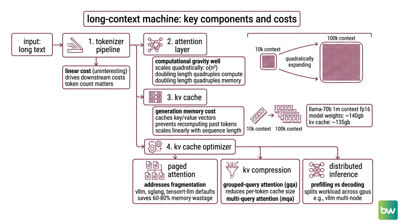
1. Tokenizer and input pipeline. Long inputs hit a tokenizer first, and the cost of tokenization is linear and uninteresting. What matters is that token count, not character count, drives every downstream cost. A 1M-token window is a 1M-token billing surface.

2. Attention layer. Self-attention compute and memory scale as O(n²) in sequence length — doubling the context length quadruples the attention compute and the peak attention memory (FlashAttention paper). This is the gravity well. Every other component in this stack is engineered around it.

3. KV cache. During generation, the model caches the keys and values of every previous token so that each new token only needs to attend, not recompute. The cache is linear in sequence length per layer, but with realistic models it is enormous. For a Llama-70B baseline at 1M context in FP16 with no compression, the KV cache is around 135 GB — larger than the roughly 140 GB FP16 model weights themselves (Introl Blog). Proprietary providers like Gemini and Claude do not publish per-token cache size, but the same scaling shape applies.

4. KV cache optimizer. The naive cache is no longer how production systems run. As of 2026, vLLM, SGLang, and TensorRT-LLM all run paged attention by default; without it, 60–80% of KV cache memory is wasted on fragmentation (DigitalApplied). On top of paging, two compression families compete: grouped-query attention (GQA), which compresses 4–8×, and DeepSeek’s Multi-head Latent Attention (MLA), which uses low-rank projection to compress 7–14× (MarkTechPost).

5. Prompt cache. A separate, externally visible cache: prefixes that repeat across requests are stored and reused. Anthropic and Google both expose this as a 90% discount on cached input tokens (PromptHub). Gemini’s explicit caching adds storage at $1 per 1M tokens per hour with a 32,768-token minimum (Gemini API Docs). Prompt caching is what makes a 1M-token system prompt economically survivable across many user turns.

Compatibility note for the long-context stack:

• FP16 KV cache, no compression: Effectively deprecated as a 2026 default. Treat it as the worst-case math, not a recommendation. Production deployments use paged attention plus GQA or MLA plus KV quantization.
• Per-token KV size for closed models: Not publicly disclosed for Gemini, Claude, or GPT. The 135 GB / Llama-70B figure is the canonical open-weights anchor — useful for shape, not for billing math.

A long-context model’s “window size” — 200K on standard Claude, 1M in beta on Opus 4.6 and Sonnet 4.6, 2M generally available on Gemini 1.5 Pro (Claude API Docs; Google Developers Blog) — is the headline number. The five components above are why each additional zero on that number costs what it costs.

The RAG machine: retrieval, indexes, and the cost of choosing wrong

RAG is the architectural answer to a different question. Instead of fitting everything into the model’s attention, you do the selection yourself, ahead of time, with cheaper machinery. The model only ever sees a small slice.

The slice is where everything goes wrong. When RAG fails in production, the failure point is retrieval roughly 73% of the time, not generation (Lushbinary). That distribution is the most important fact in this section, because it tells you which components deserve scrutiny.

What are the parts of a RAG pipeline that compete with long-context models?

A production RAG pipeline has two phases, each with its own components.

Build-time pipeline:

1. Ingestion — pulling source documents from wherever they live.
2. Chunking — splitting documents into retrievable units. Production systems hover at roughly 512–1024 tokens per chunk with 10–25% overlap. Chunk too small, you lose context; chunk too large, you dilute the embedding.
3. Embedding — running each chunk through an embedding model that maps text to a vector in some learned semantic space. The embedding model is a separate model from the generator, with its own cost and latency.
4. Indexing — storing those vectors in a structure designed for approximate nearest-neighbor search.

Runtime pipeline:

5. Query embedding — the user’s question goes through the same embedding model as the chunks.
6. Similarity search — the query vector is compared against the index. Two algorithms dominate: HNSW, a multi-layer graph that is the production default, and IVF, a cluster-based method that uses less memory on massive datasets (Core Systems). Vendors differ in which one is the default — Weaviate uses HNSW; Qdrant uses HNSW with scalar and product quantization; Pinecone combines HNSW and IVF; pgvector now offers both IVFFlat and HNSW.
7. Hybrid scoring — modern stacks rarely use vector similarity alone. Sparse Retrieval runs in parallel via BM25, and the two ranked lists are fused. The 2026 standard is Reciprocal Rank Fusion or learned score combiners; Weaviate’s BlockMax WAND with Relative Score Fusion is the most mature native hybrid (Core Systems).
8. Top-K selection and generation — the highest-ranked chunks are concatenated into the prompt and the generator model produces an answer.

The thing to notice is that this is a pipeline, not a layer. Every stage has its own accuracy, its own latency, its own way to fail silently. The vector index can return a chunk that is semantically close but factually wrong. The chunker can split a sentence across two chunks so that neither one alone answers the query. The embedding model can collapse a critical distinction into the same point in latent space.

This is also why RAG Evaluation and RAG Guardrails And Grounding are not optional layers added on top of RAG. They are the only way to know which of those eight stages is broken when an answer is wrong.

The shared substrate: what you need to know before choosing

The two stacks are different machines, but the choice between them is not made in isolation. The selection depends on facts about your data, your traffic, and your evaluation discipline. Skipping any of them turns the comparison into a religious argument.

What do you need to understand before choosing between long-context and RAG?

Four prerequisites determine whether the comparison is even meaningful for your workload.

Recall behavior across position. Long-context models do not attend uniformly to their window. Liu et al.’s 2023 “Lost in the Middle” study found that performance is highest when relevant information sits at the start or end of the context, and degrades sharply when it sits in the middle. The 2025–2026 frontier has eaten into that finding — Claude reaches 78.3% on MRCR v2, against Gemini’s 26.3% and the prior best Claude score of 18.5% (Claude5 Hub) — but the U-shaped recall curve has not been fully eliminated, especially on harder multi-fact tasks. Treat “lost in the middle” as the failure-mode framing, not the latest numbers.

Evaluation surface. Long-context evaluation is its own subdiscipline: NIAH (needle-in-a-haystack), RULER (synthetic, configurable length and complexity), MRCR (multi-round coreference recall), and GraphWalks each measure something different (Snorkel AI). RAG evaluation is different again — retrieval precision, faithfulness, answer relevance. If you cannot articulate which benchmark family matches your task, you are not yet ready to compare architectures; you are picking based on demos.

Cost shape, not cost level. Long-context queries cost in inference compute and KV memory; the cost rises with the prompt length, every request, regardless of repetition. RAG queries cost in pipeline latency and infrastructure, but the per-query payload is small. A workload with high prompt repetition (a single legal doc, queried by 1,000 users) inverts the comparison once prompt caching enters the picture. As of 2026, indicative figures from the market scan put long-context queries at 30–60 seconds and roughly 1,250× the per-query cost of RAG, but those numbers vary 10× across providers and prompt structures — they are an order-of-magnitude anchor, not a quote.

Update cadence. A long-context model carries the documents you paste in for exactly one inference pass. If your knowledge base changes daily, that is fine — paste fresh, every time. If it changes hourly across millions of users, paying that cost on every request is wasteful, and you want a vector index that can be updated incrementally.

What the components predict

Once you can name the parts, the trade-offs are no longer mysterious. They are predictions you can make before you run the workload.

• If your prompt repeats heavily across users, the prompt cache flattens the long-context cost curve, and RAG’s per-query overhead starts to look expensive instead of cheap.
• If the relevant information is buried mid-context across a 1M-token window, expect the U-shaped recall curve to bite — even with frontier 2026 models, a hard multi-fact query will not be uniformly answered.
• If your workload has retrieval misses on more than a small fraction of queries, RAG’s headline latency advantage is irrelevant; you are mostly measuring how fast you can produce a wrong answer.
• If your knowledge base updates faster than you can re-prompt, the vector index is doing work the long-context window cannot do at all without periodic re-pasting.

The 2026 default in serious production systems is not a winner-takes-all answer. It is hybrid: RAG retrieves, and a long-context model synthesizes the retrieved bundle plus any conversation history inside its window. Both stacks contribute their components, and the comparison stops being either/or.

Rule of thumb: Long-context pays per token, every request. RAG pays per pipeline stage, all the time. Pick the cost shape that matches how your traffic actually behaves.

When it breaks: Long-context degrades on mid-context recall and on workloads with low prompt repetition, where the KV cache is rebuilt for nothing. RAG degrades when retrieval misses dominate generation errors — and a vector index cannot fix a retrieval miss it does not know it made.

A connection most teams miss

The two stacks share more components than they advertise. The long-context KV cache and the RAG vector index are both engineered around the same physical fact: attention is expensive, so most of your engineering effort goes into deciding what not to attend to. Paged attention, GQA, MLA, HNSW, IVF, BM25, RRF — these are all answers to the same question, asked at different layers of the stack.

That is why the architecture argument feels so circular. The two machines are solving the same problem with different parts. The interesting question is not which one wins, but which combination of these components matches the shape of your workload — and whether you have the evaluation discipline to tell.

The Data Says

Long-context and RAG are component-list architectures, not opposing philosophies. The long-context stack pays its bill inside attention and the KV cache; the RAG stack pays its bill across an eight-stage pipeline where retrieval is the dominant failure point. The 2026 production answer is hybrid, because the components compose.