How to Build and Benchmark a Vector Index with FAISS, ScaNN, and DiskANN in 2026
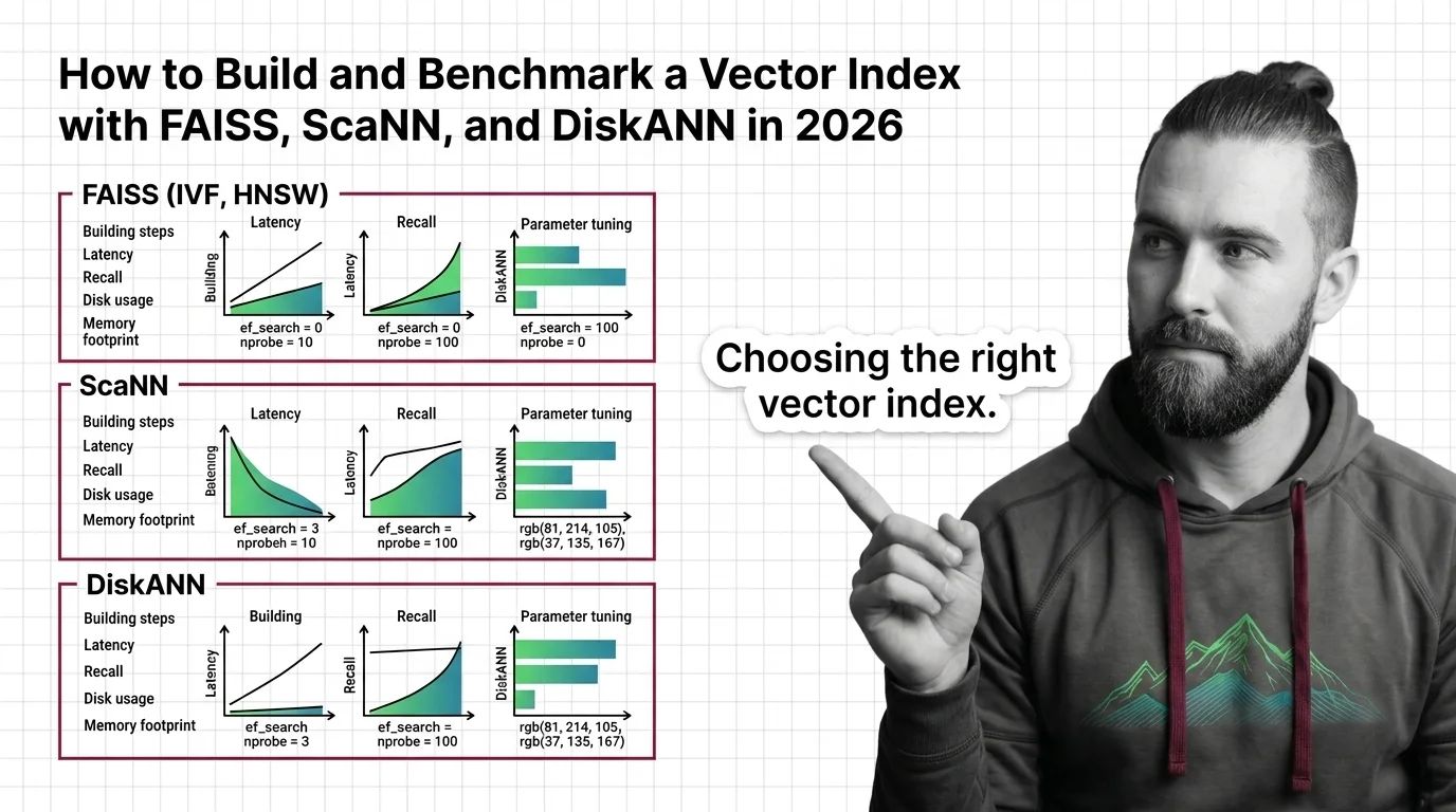
Table of Contents
TL;DR
- Choose your index type by dataset size and latency budget — not by popularity
- Tune nprobe and ef_search before adding hardware — parameter tuning is cheaper than GPU hours
- Benchmark on your actual data with ANN-Benchmarks before committing to any library
You shipped a Vector Indexing pipeline last quarter. Flat index, brute-force search, worked fine on 50K vectors. Then your dataset hit two million and p99 latency blew past 200ms. The retrieval layer that powered your RAG app just became its bottleneck. Same embeddings, same queries — the index architecture was the problem all along.
Before You Start
You’ll need:
- An AI coding tool (Claude Code, Cursor, or Codex)
- A dataset of Embedding vectors — or a plan to generate them
- Working knowledge of Similarity Search Algorithms and distance metrics (L2, cosine, inner product)
This guide teaches you: How to decompose the vector index decision into four layers — architecture, parameters, build sequence, and benchmarking — so your AI tool generates a working, tuned index instead of a demo that collapses at scale.
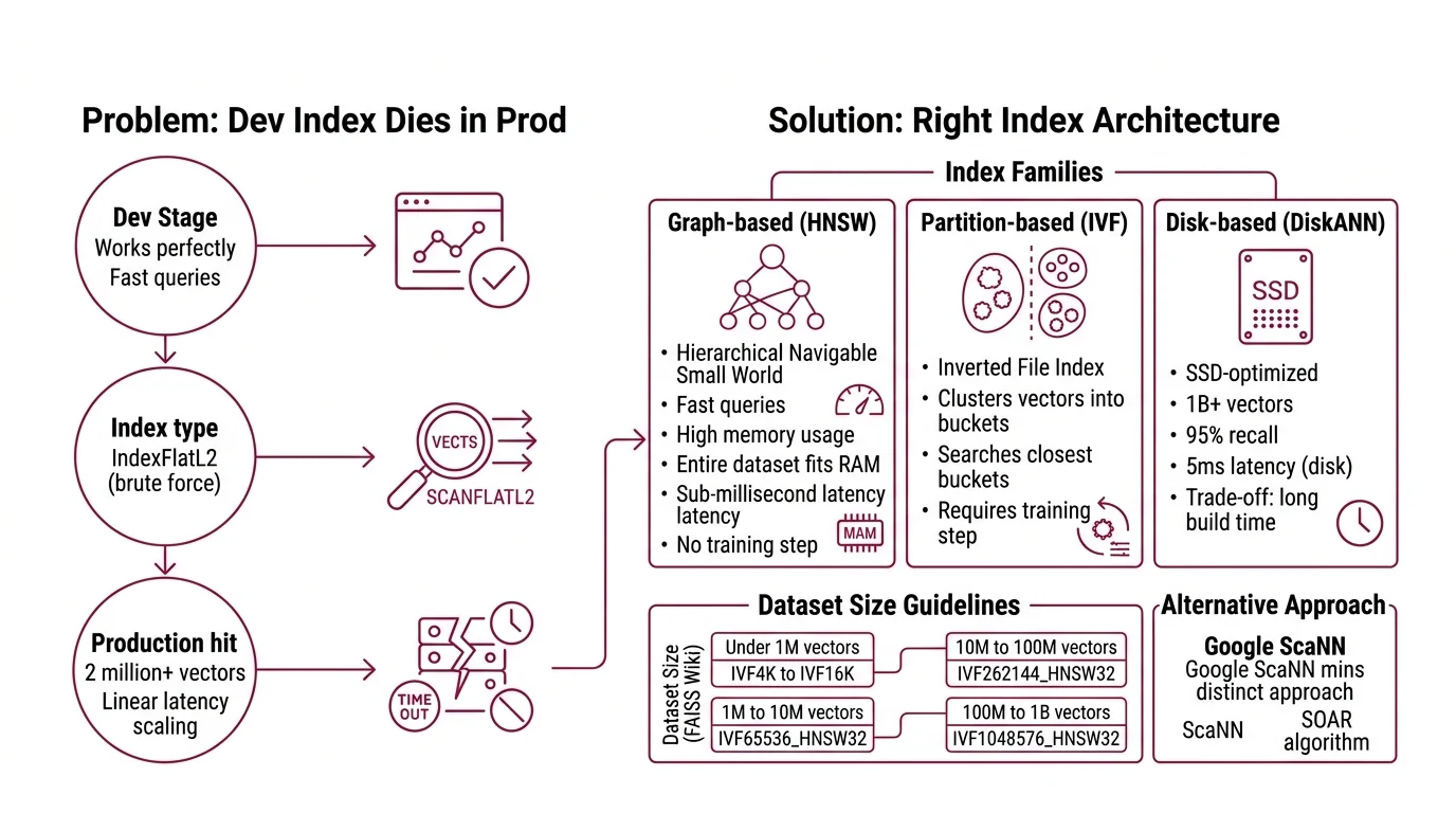
The Index That Worked in Dev and Died in Prod
Here’s the pattern. Developer grabs
Faiss because everyone uses it. Picks IndexFlatL2 because it’s the first example in the docs. Ships to staging. Works perfectly on the test set — fast, accurate, no complaints.
Production hits. Two million vectors. Ten million. Query latency goes linear because flat search checks every single vector on every single query. No index structure, no shortcuts — just brute arithmetic that scales with your data. It worked for the Tuesday demo. By Thursday, the data team doubled the corpus and every downstream service timed out.
The fix was never “add more RAM.” It was choosing the right index architecture before writing a single line of code.
Step 1: Match Your Index Architecture to Your Data
Three families of indexes cover most production workloads. Each trades a different resource for search speed.
HNSW (Hierarchical Navigable Small World): Graph-based. Fast queries, high memory. Best when your entire dataset fits in RAM and you need sub-millisecond latency. No training step required — build time scales with dataset size, but there’s no separate training phase.
IVF (Inverted File Index) (Inverted File Index): Partition-based. Clusters vectors into buckets, then searches only the closest buckets at query time. Requires a training step on representative data. The index choice is a dataset-size decision, not a preference.
FAISS guidelines map dataset size directly to index type (FAISS Wiki):
- Under 1M vectors: IVF with K = 4sqrt(N) to 16sqrt(N)
- 1M to 10M vectors: IVF65536_HNSW32
- 10M to 100M vectors: IVF262144_HNSW32
- 100M to 1B vectors: IVF1048576_HNSW32
Disk-based ( DiskANN): SSD-optimized. Handles up to one billion vectors with 95% recall at 5ms latency using disk storage instead of RAM (Microsoft Research). The trade-off: build time is measured in hours, not minutes.
ScaNN takes a different path. Its SOAR algorithm assigns vectors to multiple clusters simultaneously, which means faster search with smaller index structures (Google Research Blog). Strong on maximum inner product search workloads. As of August 2025, ScaNN 1.4.2 is the latest published release — check for newer versions before building.
The Architect’s Rule: If your dataset fits in RAM, start with HNSW. If it doesn’t, stop and evaluate DiskANN before scaling your memory budget.
Step 2: Lock Down Your Search Parameters
The index type gets you in the ballpark. Parameters determine whether you hit your recall and latency targets.
nprobe (IVF indexes): Controls how many clusters FAISS searches per query. Default is 1 — which means FAISS ignores all but one cluster out of potentially thousands (FAISS Wiki). Search time scales roughly linearly with nprobe. Start at 10. Measure recall. Increase until you hit your target, then stop.
ef_search (HNSW): Controls search depth in the graph. Higher values mean more nodes visited, better recall, slower queries. For IVF_HNSW coarse quantizers, set this via quantizer_efSearch.
Product Quantization (PQ): Compresses vectors to M-byte codes per vector. Typical M values stay at 64 or below. OPQ pre-processing improves quality by rotating vectors before quantization — worth the extra build step when memory is tight.
Context checklist for your AI tool:
- Distance metric: L2, inner product, or cosine
- Target recall@10 (start with 0.95)
- Maximum p99 latency in milliseconds
- Available RAM per index shard
- Dataset dimensionality and vector count
- Whether you need real-time inserts or batch-only
The Spec Test: If your context doesn’t specify the distance metric, the AI will default to L2 when your embeddings might need cosine similarity. One wrong parameter. Wrong results on every query.
Step 3: Build the Index Pipeline
Order matters. Each component depends on the previous one’s contract.
Build order:
- Embedding generation first — because index dimensions and distance metrics are locked to your embedding model. Changing the model later means rebuilding everything downstream.
- Index construction second — training (IVF) or graph building (HNSW/DiskANN). This is the compute-intensive step that benefits from batching.
- Query interface last — wraps the index with parameter tuning, batching logic, and error handling.
For each component, your AI tool must know:
- What it receives (inputs: vector dimensions, batch size, data format)
- What it returns (outputs: index file path, top-K results with distances)
- What it must NOT do (constraints: memory ceiling, no silent fallbacks on corrupted data)
- How to handle failure (error cases: wrong dimensions, missing index file, OOM during training)
Installation note: The FAISS pip CPU package (v1.13.2 as of December 2025) lags the latest GitHub release. For v1.14.1 features — RaBitQ fast scan, ARM SVE support, dynamic dispatch — install from conda or build from source (FAISS GitHub). GPU support requires the faiss-gpu-cuvs package via NVIDIA cuVS.
Step 4: Benchmark Before You Commit
Gut feeling is not a benchmark. ANN-Benchmarks gives you reproducible recall-vs-QPS curves on standard datasets.
What ANN-Benchmarks provides: A Docker-based framework covering 40+ algorithms, run on standardized hardware — AWS r6i.16xlarge, single CPU (ANN-Benchmarks GitHub). Standard datasets include SIFT-1M (128 dimensions, Euclidean), GloVe (25 to 200 dimensions, Angular), and GIST (960 dimensions). Pick the dataset closest to your embedding profile.
What to measure:
- Recall@10 at your target QPS — the only number that matters for production
- Memory footprint per million vectors
- Index build time (minutes for HNSW, hours for DiskANN at scale)
- Query latency distribution: p50, p95, p99 — not averages
ANN-Benchmarks won’t tell you how your specific data distribution affects recall. Benchmark datasets are clean and uniform. Your production data probably isn’t. Run the standard benchmarks first to validate your index choice, then re-run on a representative sample of your actual vectors to validate the parameters.
Common Pitfalls
| What You Did | Why It Failed | The Fix |
|---|---|---|
| Used IndexFlatL2 beyond 100K vectors | Brute-force scales linearly — every query touches every vector | Switch to IVF or HNSW at the dataset-size threshold |
| Left nprobe at default (1) | Searched one cluster out of thousands — recall near zero | Set nprobe to 10 and tune upward against your recall target |
| Picked HNSW for 500M vectors | Graph index consumed all available RAM | Evaluate DiskANN or IVF with PQ compression |
| Benchmarked on SIFT-1M only | Standard dataset doesn’t match your embedding distribution | Run ANN-Benchmarks first, then benchmark on your data |
| Used DiskANN C++ examples from pre-2025 | Rust rewrite since v0.45.0 replaced the C++ API entirely | Use diskannpy 0.7.0+ with the unified index.search() method |
Compatibility notes:
- DiskANN API change (v0.47.0+): The Rust rewrite unified the search API —
index.search()replaces individual search methods, and parameters are now the first argument. C++ code lives on the legacycpp_mainbranch only. Verify diskannpy examples against current docs before building (DiskANN GitHub).
Pro Tip
Every index configuration is a hypothesis. Treat it like one. Write your target recall, latency budget, and memory limit as assertions before you pick a library — then let the benchmark prove or disprove them. The teams that ship reliable vector search are the ones that specified “95% recall@10 under 5ms at 10M scale” before they wrote their first import faiss, not after.
Frequently Asked Questions
Q: How to build a vector search index with FAISS IVF and HNSW step by step? A: Train the IVF quantizer on a representative sample, build the index with your full dataset, then layer HNSW as the coarse quantizer for faster cluster selection. Key gotcha: a biased training sample produces clusters that miss entire query regions — sample uniformly across your data distribution.
Q: How to choose between HNSW IVF and product quantization for your dataset size and latency requirements? A: HNSW for sub-million in-memory speed, IVF for partitioned search at scale, PQ when memory is the binding constraint. Combine them — IVF_HNSW with PQ compression covers the 10M-to-1B range. The variable most teams miss: whether the workload needs real-time inserts or batch-only rebuilds.
Q: How to tune FAISS nprobe and ef_search parameters for optimal recall vs speed tradeoff? A: Start nprobe at 10, double it, measure recall@10 at each step. Stop when recall plateaus — more probes after that point burn CPU for negligible gain. Apply the same doubling strategy to ef_search for HNSW depth. Log every configuration so you can replay the tuning curve.
Q: How to benchmark vector index performance using ANN-Benchmarks in 2026? A: Clone the repo, pick the dataset closest to your embedding profile, run via Docker. The recall-vs-QPS plot is your decision artifact. One caveat: the ANN-Benchmarks website plots may lag behind the actual repo data — run locally for current numbers.
Your Spec Artifact
By the end of this guide, you should have:
- Index architecture map — dataset size bracket mapped to index type and parameter ranges
- Parameter constraint list — nprobe, ef_search, PQ dimensions, distance metric, recall target, latency budget
- Benchmark validation criteria — target recall@K at target QPS, memory ceiling, build time limit
Your Implementation Prompt
Paste this into your AI coding tool after filling in the bracketed values. It encodes the decision framework from Steps 1 through 4 — your decomposition, your constraints, your validation criteria.
Build a vector search index pipeline with the following specifications:

DATASET:
- Vector count: [number of vectors, e.g. 5000000]
- Dimensions: [embedding dimensions, e.g. 768]
- Distance metric: [L2 / inner_product / cosine]
- Data format: [numpy .npy / memory-mapped / streaming]

INDEX ARCHITECTURE (from Step 1 size brackets):
- Library: [faiss / scann / diskann]
- Index type: [IVF{nlist}_HNSW32 / HNSW / DiskANN graph]
- Reason: [dataset fits in RAM / exceeds RAM / needs SSD-backed search]

PARAMETERS (from Step 2 checklist):
- nprobe: [starting value, e.g. 10]
- ef_search: [starting value, e.g. 64]
- PQ compression: [M value, e.g. 32, or "none"]
- Target recall@10: [e.g. 0.95]
- Max p99 latency: [e.g. 5ms]
- Max RAM per shard: [e.g. 16GB]

BUILD ORDER (from Step 3):
1. Embedding ingestion — input: [source format], output: numpy array of [dims]d float32
2. Index training and construction — input: training vectors, output: serialized index file
3. Query interface — input: query vector, output: top-K IDs + distances

CONSTRAINTS:
- Incremental inserts required: [yes / no]
- Error handling: reject queries with wrong dimensions, return empty result set on corrupted index, log OOM during training
- Installation: [pip faiss-cpu / conda faiss-gpu-cuvs / diskannpy / scann]

VALIDATION (from Step 4):
- Benchmark dataset: [SIFT-1M / GloVe / custom representative sample]
- Pass criteria: recall@10 >= [target] at >= [target QPS] queries/sec
- Report: p50, p95, p99 latency, memory footprint, build time
Ship It
You now have a framework for choosing, tuning, and proving a vector index works — before it hits production. The decision is no longer “which library is popular.” It’s “which architecture meets my recall target within my memory and latency budget.” That question has a measurable answer.
AI-assisted content, human-reviewed. Images AI-generated. Editorial Standards · Our Editors