How to Build an LSTM in PyTorch and Where RNNs Still Outperform Transformers in 2026
Table of Contents
TL;DR
- RNNs still win in three domains: edge devices under 30 KB RAM, streaming anomaly detection, and low-data time series — transformers are overkill there
- Specify the temporal contract first — sequence length, hidden state size, and prediction horizon — before touching any model code
- Use the Decompose-Specify-Build-Validate loop to get your AI coding tool to generate a working LSTM on the first pass
Your AI coding tool just generated a transformer for a vibration sensor running on a microcontroller with 29 KB of RAM. The model is 400 MB. The device has no GPU. You asked for “a time series anomaly detector” and got a solution that cannot physically run on the target hardware. The prompt never mentioned the constraint.
Before You Start
You’ll need:
- An AI coding tool — Claude Code, Cursor, or Codex
- Familiarity with Recurrent Neural Network architecture and Neural Network Basics for LLMs
- A clear picture of your deployment target — device, memory budget, latency requirement
This guide teaches you: how to decompose an LSTM build into specifiable components so your AI tool generates a model that fits your constraints on the first try.
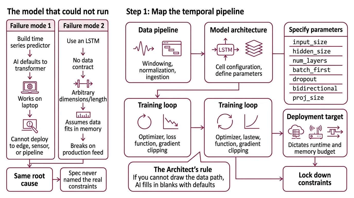
The Model That Could Not Run
Two failure modes show up constantly.
First: you prompt “build me a time series predictor” and the AI defaults to a transformer. Training bias. The model works on your laptop. It cannot deploy to the edge device, the embedded sensor, or the streaming pipeline where you actually need it.
Second: you specify “use an LSTM” but skip the data contract. The AI picks arbitrary hidden dimensions, guesses at sequence length, and generates a training loop that assumes your data fits in memory. It worked on the tutorial dataset. It breaks on your production feed.
Both failures have the same root cause. The spec never named the real constraints.
Step 1: Map the Temporal Pipeline
An RNN build has distinct components. Each one is a separate concern for your AI tool.
Before you prompt anything, understand what you are assembling:
- Data pipeline — ingestion, windowing, normalization. This component turns raw signals into fixed-length sequences the model can consume. The windowing strategy determines what the model sees.
- Model architecture — the LSTM cell configuration itself.
torch.nn.LSTMin PyTorch takesinput_size,hidden_size,num_layers,batch_first,dropout,bidirectional, andproj_size(PyTorch Docs). Each parameter is a constraint your specification must lock down. - Training loop — optimizer, loss function, learning rate schedule, early stopping. This is where Backpropagation Through Time happens and where gradient clipping prevents exploding gradients.
- Deployment target — where the trained model runs. A cloud API, an edge device, a streaming pipeline. The target dictates quantization, runtime, and memory budget.
The Architect’s Rule: If you cannot draw the data path from raw input to prediction output in these boxes, your AI tool will fill in the blanks with defaults. Its defaults are not your requirements.
Step 2: Write the Temporal Contract
This is where most LSTM builds go sideways. The AI needs exact numbers, not descriptions.
Context checklist:
- Input shape:
[batch_size, sequence_length, features]— specify all three dimensions - Hidden State size: tied to model capacity. Larger means more expressive but more memory. For edge targets, this is your primary constraint lever
- Number of LSTM layers: stacked layers add capacity but increase training time and memory
- Output contract: single-step prediction, multi-step forecast, or classification logits
- Quantization plan: FP32 for training, but does your deployment target need INT8? LSTM quantization to INT8 causes measurable accuracy drops on microcontrollers (Saha & Samanta) — specify acceptable accuracy loss upfront
- Memory budget: total RAM available on the deployment target, minus OS and application overhead
- Framework version: PyTorch 2.11.0, the current stable release as of January 2026
The Spec Test: If your context file does not specify the hidden state size, your AI tool will default to 256 or 512 — the numbers from every tutorial. For an Arduino with 29 KB of RAM, that model will not fit. Name the number.
Step 3: Sequence the Build
Order matters. Each component depends on decisions made in the previous one.
Build order:
- Data pipeline first — because every downstream decision depends on input shape. Window size determines sequence length. Feature count determines input_size. Normalization determines scale. Get these wrong and nothing else matters.
- Model architecture second — because it consumes the data pipeline’s output shape. Hidden size and layer count are constrained by deployment memory. Lock these after you know your data shape and your memory budget.
- Training loop third — because optimizer choice and gradient clipping depend on architecture depth. Deeper stacks need more aggressive clipping. Bidirectional models need different batch handling.
- Deployment wrapper last — because it takes the trained model and fits it to the runtime. ExecuTorch v1.2 provides a 50 KB base runtime with support for Apple, Qualcomm, ARM, and MediaTek hardware (ExecuTorch Docs). Specify the target backend before export.
For each component, your context must specify:
- What it receives (input shape and type)
- What it returns (output shape and type)
- What it must NOT do (no assumptions about batch size, no hardcoded paths)
- How to handle failure (what happens when a sequence is shorter than the window)
Step 4: Prove the Temporal Model Works
Validation for sequence models is different from classification. Time leaks, look-ahead bias, and non-stationary signals will pass standard test splits and fail in production.
Validation checklist:
- Walk-forward split — failure looks like: suspiciously high accuracy from data leakage. Train on months 1-6, validate on month 7, retrain on 1-7, validate on 8. Never shuffle time series.
- Hidden state reset — failure looks like: predictions that drift after the first batch. Verify the hidden state resets between sequences during inference. If it carries over, your model is cheating.
- Latency on target hardware — failure looks like: model runs in 50 ms on your laptop, 2000 ms on the ESP32. Benchmark on the actual deployment device, not your development machine. A DeepConv LSTM achieved 21 ms inference on an Arduino Nano 33 BLE Sense Rev2 with 98.24% accuracy for activity recognition (Nature Scientific Reports) — that is your reference for what is achievable.
- Quantization accuracy gap — failure looks like: significant accuracy drop after INT8 conversion. On ESP32 hardware, one study measured LSTM accuracy dropping from 89.52% (FP32) to 85.53% (INT8), while a Convolutional Neural Network maintained 95.49% to 95.36% (Saha & Samanta). Quantization hits recurrent models harder than convolutional ones. Measure before you ship.
Common Pitfalls
| What You Did | Why AI Failed | The Fix |
|---|---|---|
| “Build me a time series model” | AI defaulted to transformer — training bias | Specify “LSTM” and name the architecture constraints |
| No memory budget | AI generated a 256-hidden model that exceeds device RAM | Add target device, RAM limit, and acceptable model size |
| Skipped sequence length | AI picked 128 steps — wrong for your sampling rate | Compute window size from your data frequency and prediction horizon |
Used batch_first=False | AI followed old tutorials — your data loader assumes batch-first | Specify batch_first=True in the context file |
| No gradient clipping | Training diverges at epoch 30 with exploding gradients | Add torch.nn.utils.clip_grad_norm_ with max_norm to training spec |
Pro Tip
Every specification you write for an LSTM transfers to the next sequence model. The data contract, the windowing strategy, the deployment memory budget — these do not change when you swap the model for an xLSTM or a state-space model. The architecture is the replaceable part. The specification is the reusable part. Invest in the spec and the next model swap costs you an afternoon, not a week.
The xLSTM architecture introduces matrix memory cells that are fully parallelizable during training (Beck et al.), and a 7B parameter model is available on HuggingFace. The minLSTM variant removes hidden-state dependencies from gates entirely, training 235x faster than traditional LSTMs at sequence length 512 (Feng et al.). These are drop-in candidates when your spec is solid. Note: the xLSTM HuggingFace Transformers integration has known bugs preventing training of models smaller than 7B parameters.
Frequently Asked Questions
Q: How to build an LSTM model in PyTorch for time series prediction step by step? A: Decompose into data pipeline, model architecture, training loop, and deployment wrapper. Specify each component’s input/output contract before prompting your AI tool. The Implementation Prompt section below encodes this exact sequence with placeholders for your project constraints.
Q: When should you use an LSTM instead of a transformer in 2026? A: When your target has under 1 MB RAM, when training data is too small for a transformer to generalize, or when you need streaming inference without buffering full context windows. Edge sensors, anomaly detection, and low-data industrial time series are where LSTMs win. Transformers remain stronger for NLP.
Q: How to use RNNs for anomaly detection in time series data? A: Specify an LSTM autoencoder — the model learns to reconstruct normal patterns, and reconstruction error flags anomalies. A MIX_LSTM architecture achieved 0.984 AUC-ROC on the UNSW-NB15 intrusion detection benchmark (Nature Scientific Reports). For distributed environments, federated LSTM autoencoders enable anomaly detection across nodes without centralizing sensitive data.
Q: What are the best use cases for RNNs on edge devices with limited compute in 2026? A: Activity recognition on wearables (DeepConv LSTM: 98.24% accuracy, 29.1 KB RAM on Arduino), predictive maintenance on industrial sensors, and streaming anomaly detection on IIoT gateways. ExecuTorch v1.2 handles deployment from PyTorch to edge targets. Specify INT8 quantization tolerance early — recurrent models lose more accuracy than CNNs.
Your Spec Artifact
By the end of this guide, you should have:
- A temporal pipeline map — data pipeline, model architecture, training loop, and deployment target with explicit boundaries and data shapes flowing between them
- A constraint checklist — hidden size, sequence length, memory budget, quantization plan, and framework version, all with concrete numbers for your use case
- A validation protocol — walk-forward splits, hidden state reset checks, on-device latency benchmarks, and quantization accuracy gap measurements
Your Implementation Prompt
Paste this into Claude Code, Cursor, or Codex after filling in your constraints. Every bracketed placeholder maps to a specific item from your constraint checklist in Step 2.
Build an LSTM-based [single-step prediction | multi-step forecast | anomaly detector] using PyTorch 2.11.

DATA PIPELINE:
- Input: [your data source and format]
- Window size: [sequence_length] steps at [sampling_rate] Hz
- Features: [feature_count] channels, normalized with [min-max | z-score]
- Split: walk-forward — train on [train_period], validate on [val_period]

MODEL ARCHITECTURE:
- torch.nn.LSTM with input_size=[feature_count], hidden_size=[hidden_size], num_layers=[layer_count], batch_first=True
- Bidirectional: [True | False]
- Output layer: Linear([hidden_size], [output_size])
- Total model must fit in [memory_budget_kb] KB when quantized to [FP32 | INT8]

TRAINING:
- Optimizer: [Adam | AdamW] with lr=[learning_rate]
- Loss: [MSE | MAE | BCE]
- Gradient clipping: max_norm=[clip_value]
- Early stopping: patience=[patience_epochs] on validation loss

DEPLOYMENT:
- Target: [device name and specs]
- Runtime: [ExecuTorch | ONNX Runtime]
- Latency requirement: under [max_ms] ms per inference
- Quantization: [FP32 | INT8] — acceptable accuracy drop: [max_percent]%

VALIDATION:
- Walk-forward cross-validation, never shuffle temporal order
- Reset hidden state between sequences during inference
- Benchmark inference latency on [target device], not development machine
- Report quantization accuracy gap: FP32 vs INT8 on validation set
Ship It
You now have a framework for specifying any LSTM build — from an Arduino sensor to a cloud anomaly detector. The architecture is the easy part. The specification is what makes it work on the first try. Next time your AI tool reaches for a transformer, you will know exactly when to override that default and why.
AI-assisted content, human-reviewed. Images AI-generated. Editorial Standards · Our Editors