How to Build a Similarity Search Pipeline with FAISS, HNSWlib, and ScaNN in 2026
Table of Contents
TL;DR
- Decompose your similarity search into four layers — embedding, indexing, quantization, retrieval — and specify each one independently
- Pick your library based on hard constraints (memory budget, latency ceiling, dataset scale), not blog rankings
- Validate with recall@k and latency benchmarks before you ship, not after the on-call page fires at 3 AM
Somebody on your team typed “build me a vector search” into their AI coding tool. They got a flat brute-force index over a million Embedding vectors. It worked in dev. It ate 47 GB in staging. Nobody specified the index type, the distance metric, or the memory ceiling. The AI didn’t ask. It never does.
Before You Start
You’ll need:
- An AI coding tool (Claude Code, Cursor, or Codex)
- A working grasp of Similarity Search Algorithms and why approximate methods exist
- Your dataset size, dimensionality, and latency requirements — on paper, not in your head
This guide teaches you: how to decompose a similarity search pipeline into specifiable layers so your AI tool builds an index that survives production load.
The Index That Swallowed Your Cluster
Here’s the scene I keep finding.
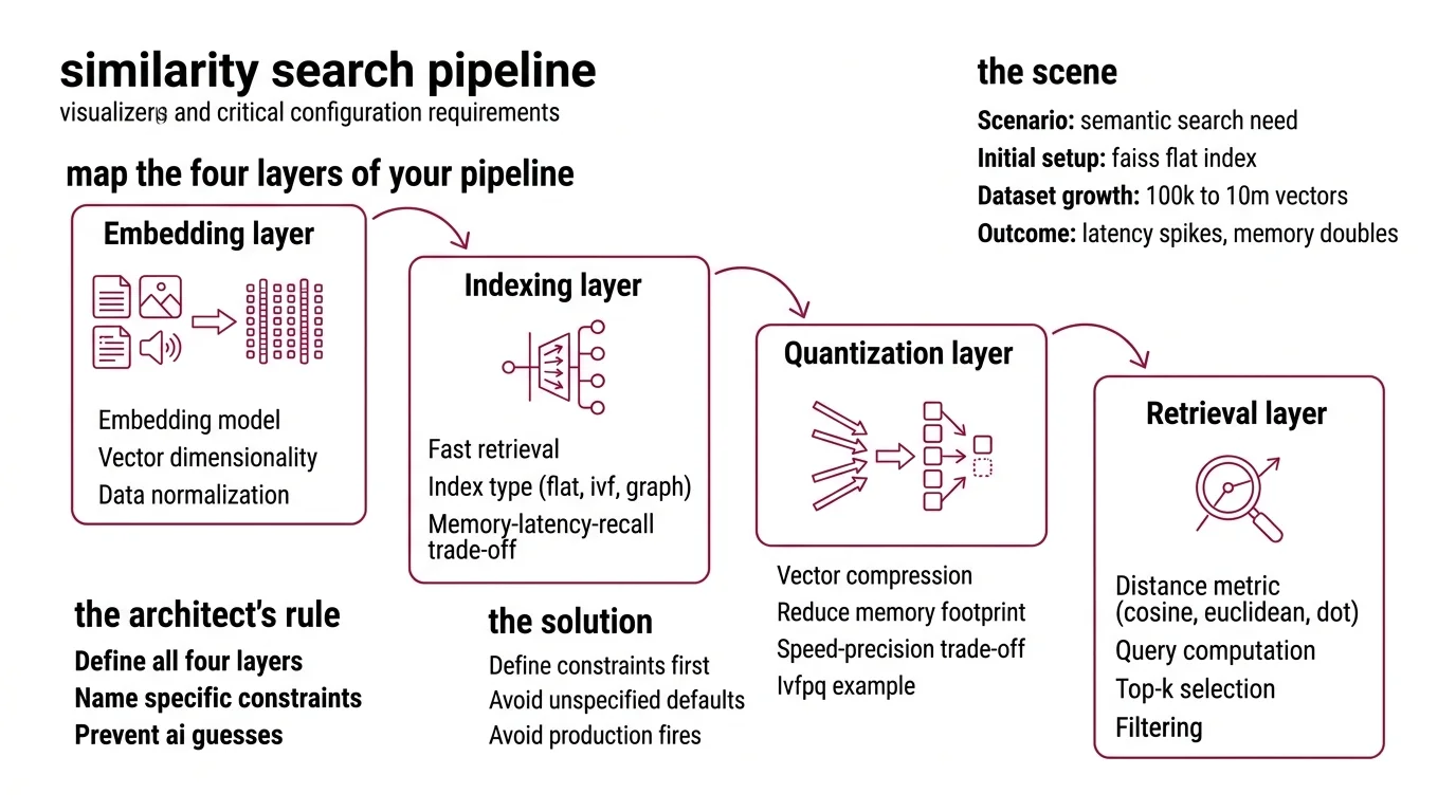
Developer needs semantic search. Reads a blog post. Picks FAISS because it had the most stars. Copies the flat index example. Ships it. The dataset grows from 100K to 10M vectors. Latency spikes. Memory doubles. The ops team gets paged.
It worked on Tuesday. On Friday, search started timing out because the dataset crossed the brute-force threshold — the point where unspecified defaults become production fires.
The fix was never “try HNSWlib instead.” The fix was specifying the constraints before writing the first line of index code.
Step 1: Map the Four Layers of Your Pipeline
Every similarity search pipeline has four layers. Miss one and the AI guesses. Those guesses will be wrong.
Your system has these parts:
- Embedding layer — converts raw data (text, images, audio) into dense vectors. You specify the model, the dimensionality, and the normalization. The AI picks nothing here. You pick everything.
- Indexing layer — organizes vectors for fast retrieval. Flat index, inverted file index, graph-based index. Each has a different memory-latency-recall trade-off. This is where most specs fail. Developers skip this and get brute-force by default.
- Quantization layer — compresses vectors to cut memory. Product Quantization can shrink your index dramatically. IVF-PQ delivers roughly 92x throughput versus a non-quantized flat index with less than ten percent recall loss (Pinecone). But you trade precision for speed. Specify that trade-off or the AI skips compression entirely.
- Retrieval layer — handles the actual query: distance computation, top-k selection, filtering. You specify the distance metric — Cosine Similarity, Euclidean Distance, or Dot Product — and the AI wires the rest.
The Architect’s Rule: If you can’t name all four layers and their constraints, the AI will fill at least two of them with defaults. Defaults that fit nobody’s production environment.
Step 2: Lock the Library to Your Constraints
Three libraries own this space. None of them is “the best.” Each one is best at something specific. Your job is matching your hardest constraint to the right tool.
FAISS (Meta) — v1.14.1, released March 2026 (FAISS GitHub). Supports Flat, IVF-Flat, IVF-PQ, HNSW, RaBitQ, and more. GPU acceleration via cuVS delivers up to 12x faster index builds and 8x lower search latency at 95% recall (Meta Engineering Blog). If you need billion-scale search on GPUs, start here.
HNSWlib — v0.8.0, released December 2024 (HNSWlib GitHub). Header-only, lightweight, fast on CPU. Supports L2, inner product, and cosine distance with AVX512 optimizations. Multi-vector document search built in. No GPU support. No quantization. As of early 2026, HNSWlib has not shipped a new release in over fifteen months — factor maintenance pace into your decision.
ScaNN (Google) — v1.4.2, released August 2025 (ScaNN PyPI). Strong on high-dimensional data. The SOAR algorithm improves indexing with learned redundancy (Google Research Blog). Dynamic updates — insert, modify, delete vectors — since v1.3.0. TensorFlow dependency is optional since v1.4.0.
The decision is not “which is best.” The decision maps constraints to capabilities:
| Constraint | FAISS | HNSWlib | ScaNN |
|---|---|---|---|
| Billion-scale datasets | IVF-PQ, GPU | Memory-limited | SOAR, tree-based |
| Lowest CPU latency | Good | Excellent | Good |
| GPU acceleration | cuVS (since v1.10) | None | Limited |
| Dynamic updates | Limited (rebuild) | In-place | Since v1.3.0 |
| Minimal dependencies | pip install | Header-only C++ | pip install |
Security & compatibility notes:
- FAISS v1.14.0 API changes: SWIG typed vectors renamed (LongVector to Int64Vector), method suffix “Ex” renamed to “_ex”, NumPy 2.0 compatibility added. Pin to v1.14.1 and verify serialization round-trips after upgrading.
- FAISS deserialization hardening: v1.14 added safety checks for untrusted index files. Do not load indexes from untrusted sources on prior versions.
- ScaNN TF dependency: TensorFlow integration is no longer default since v1.4.0. Install with
pip install scann[tf]if you need TF ops. Requires TF 2.19+ and is not backwards-compatible.
Step 3: Wire the Index Architecture
Build order matters. Get it wrong and the AI builds components that don’t connect.
Build order:
- Embedding pipeline first — because every downstream component depends on knowing the vector dimensionality and normalization. Lock this or the AI will hallucinate a dimension count.
- Index structure second — because it determines the memory-latency envelope. IVF-PQ for billion-scale, HNSW for low-latency CPU, flat for anything under a million vectors.
- Quantization layer third — because it compresses what the index stores. You can’t configure product quantization or Locality Sensitive Hashing without knowing the index type first.
- Retrieval and query interface last — because it integrates everything. Distance metric, top-k, pre-filtering, post-filtering.
For each component, your context must specify:
- What it receives (vector dimensions, data types, batch sizes)
- What it returns (ranked results, distances, metadata)
- What it must NOT do (no unbounded memory allocation, no blocking queries during rebuilds)
- How to handle failure (index corruption, OOM, dimension mismatch)
The Spec Test: If your context doesn’t specify the distance metric, the AI will default to L2 Euclidean when your embeddings need cosine similarity. Normalized vectors hide this bug until you hit edge cases with near-zero magnitude vectors.
Step 4: Prove Your Pipeline Survives Load
You built an index. Now prove it works at your actual scale. Not your demo scale.
Validation checklist:
- Recall@10 against ground truth — failure looks like: relevant results missing, low recall despite fast queries. Run your evaluation against standard benchmarks — ANN-Benchmarks evaluates algorithms across datasets including glove-100 and sift-128 at k=10 (ANN-Benchmarks). Your index should match published recall curves for your chosen algorithm.
- Latency at p99 under concurrent load — failure looks like: median latency is fine, tail latency blows past your SLA. Flat indexes degrade linearly. HNSW degrades gracefully. IVF can spike during nprobe tuning.
- Memory footprint at target scale — failure looks like: index fits in dev, OOMs in staging. Quantized indexes use a fraction of the memory, but measure the actual compression ratio. Not the theoretical one.
- Index build time — failure looks like: rebuilding takes six hours, your data refreshes every two. GPU-accelerated FAISS builds cut this, but only if your spec includes GPU requirements.
Common Pitfalls
| What You Did | Why AI Failed | The Fix |
|---|---|---|
| “Build me vector search” | Too vague — AI picked flat index for 50M vectors | Specify dataset scale and latency ceiling |
| No distance metric stated | AI defaulted to L2 on normalized embeddings | State cosine, L2, or inner product explicitly |
| Skipped quantization spec | Index consumed full float32 per dimension | Specify memory budget and acceptable recall loss |
| Picked library from a blog | Wrong tool for your actual constraints | Use the constraint table from Step 2 |
Pro Tip
Your index type is a contract. When you spec IVF-PQ with nlist=4096 and m=32, you lock a precision-memory trade-off. Change one parameter and the entire recall-latency curve shifts. Spec the parameters and the trade-off. The AI respects explicit constraints. It never infers them.
Frequently Asked Questions
Q: How to implement cosine similarity search with FAISS step by step in Python?
A: Normalize your vectors to unit length first, then use IndexFlatIP — on normalized vectors, inner product equals cosine similarity. Specify L2-normalization in your embedding pipeline, not inside FAISS. Common trap: using IndexFlatL2 and expecting cosine results.
Q: How to choose between FAISS, HNSWlib, and ScaNN for a similarity search project in 2026? A: Start with your hardest constraint. GPU acceleration required? FAISS. Minimal dependencies and fast CPU search? HNSWlib. Dynamic inserts and deletes on high-dimensional data? ScaNN since v1.3.0. Watch HNSWlib’s maintenance pace and ScaNN’s self-reported benchmarks.
Q: How to build a billion-scale approximate nearest neighbor index with product quantization and IVF?
A: Spec an IVF-PQ index in FAISS with a large representative training sample. Set nlist proportional to your dataset’s square root and tune nprobe for the recall-speed trade-off at query time. Both are constraints you spec upfront — not numbers you guess at deployment.
Your Spec Artifact
By the end of this guide, you should have:
- A four-layer pipeline decomposition (embedding, indexing, quantization, retrieval) with constraints locked for each layer
- A library selection rationale tied to your three hardest constraints — not a blog recommendation
- A validation checklist with recall, latency, memory, and build-time targets specific to your dataset scale
Your Implementation Prompt
Paste this into Claude Code, Cursor, or Codex after filling in your constraints. Every bracket maps to a decision from Steps 1 through 4.
Build a similarity search pipeline with the following specification:

EMBEDDING LAYER:
- Model: [your embedding model, e.g., text-embedding-3-large]
- Dimensions: [output dimension count]
- Normalization: [L2-normalize / none]

INDEX LAYER:
- Library: [FAISS / HNSWlib / ScaNN]
- Index type: [Flat / IVF-Flat / IVF-PQ / HNSW / SOAR]
- Dataset size: [current vector count and expected 12-month growth]
- Distance metric: [cosine / L2 / inner product]

QUANTIZATION LAYER:
- Method: [product quantization / scalar quantization / none]
- Subquantizers (m): [count, must divide dimensions evenly]
- Training set size: [large representative sample for IVF-PQ training]
- Acceptable recall loss: [percentage ceiling, e.g., <5%]

RETRIEVAL LAYER:
- Top-k: [result count per query]
- nprobe (IVF only): [partitions to search, e.g., 64]
- Pre-filtering: [metadata filters before search / none]
- Post-filtering: [score threshold / none]

CONSTRAINTS:
- Memory ceiling: [e.g., 16 GB per node]
- Latency target: [p99 in ms, e.g., <50ms]
- Concurrent queries: [expected QPS]
- Index rebuild frequency: [e.g., every 6 hours]
- GPU required: [yes/no, GPU model if yes]

VALIDATION:
- Benchmark recall@10 against brute-force ground truth on [your dataset]
- Measure p99 latency under [concurrent query count] load
- Verify memory stays under [ceiling] at [target vector count]
- Confirm index build completes within [rebuild window]
Ship It
You now have a framework for specifying similarity search pipelines that an AI tool can actually build correctly. Four layers. Hard constraints at every boundary. Measurable validation before anything hits production. The next time someone says “just use FAISS,” you’ll know the right question: for what constraints?
AI-assisted content, human-reviewed. Images AI-generated. Editorial Standards · Our Editors