How to Apply Scaling Laws and Chinchilla-Optimal Ratios to LLM Training Decisions in 2026
Table of Contents
TL;DR
- The Chinchilla 20:1 token-to-parameter ratio optimizes training compute — not inference cost, which now dominates total spend
- Use C ≈ 6ND to map your compute budget, then adjust the ratio based on how many inference requests your model will serve
- Scaling laws are empirical fits, not physics — validate every estimate against published benchmarks before committing GPU-hours
You have a compute budget. You have a target capability. You Google “Chinchilla optimal,” find the 20:1 ratio, and size your model accordingly. Three months later, your model works — but serving it costs four times what you planned. The ratio was right for 2022. Your inference bill is from 2026.
Before You Start
You’ll need:
- A defined compute budget in GPU-hours or FLOPs
- Familiarity with Scaling Laws and how Power Law relationships govern model performance
- A clear deployment target — batch processing, real-time API, or edge inference
This guide teaches you: How to translate scaling law equations into a concrete model-size and data-size decision that accounts for both training efficiency and inference cost.
The 20:1 Ratio That Breaks Your Inference Budget
Here’s the scenario I see repeated across teams.
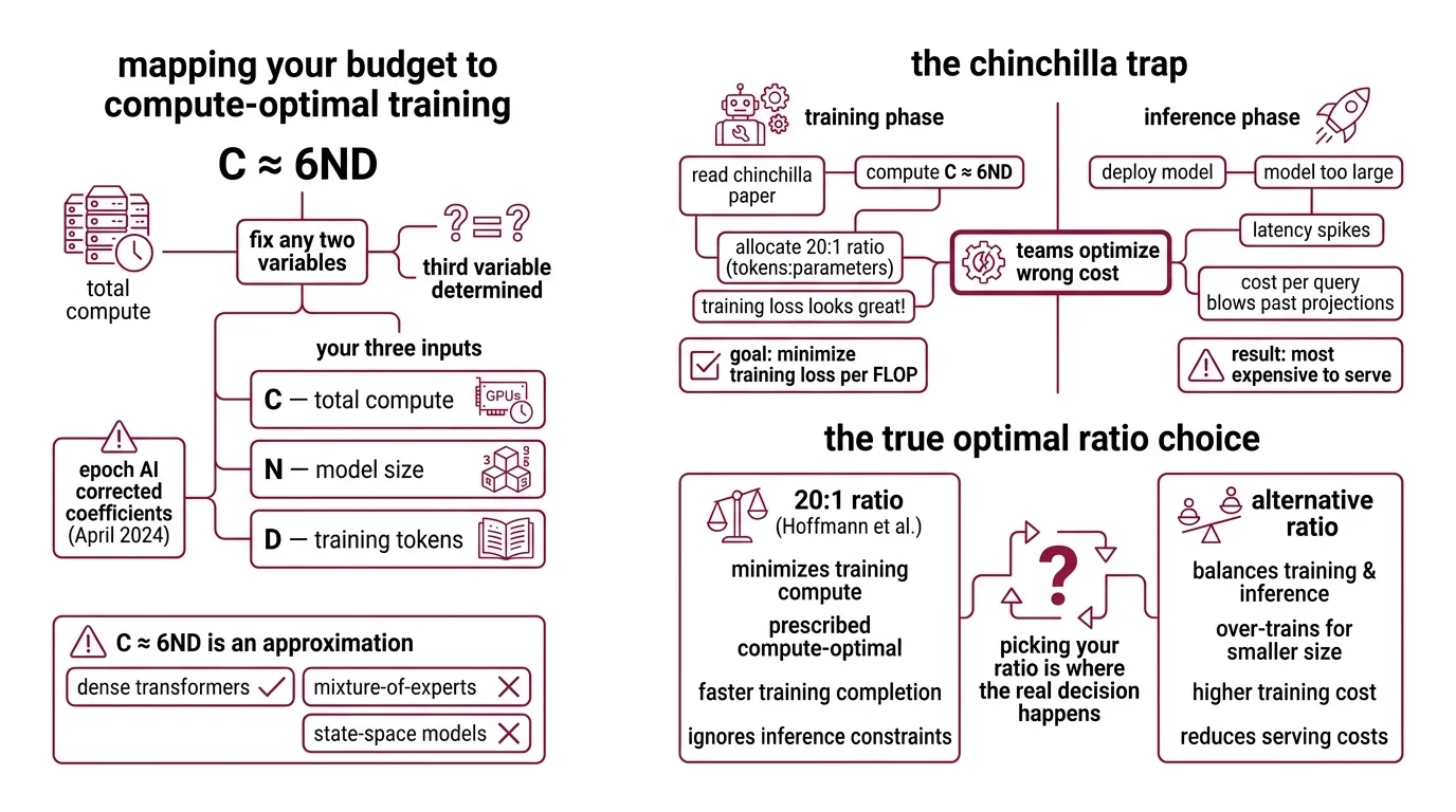
An ML team reads the Chinchilla paper. They compute C ≈ 6ND. They allocate parameters and tokens at the 20:1 ratio. Training loss looks great. Then they deploy — and the model is too large for their inference infrastructure. Latency spikes. Cost per query blows past projections.
The 20:1 ratio from Hoffmann et al. minimizes training loss per FLOP. It says nothing about what happens after training — when inference demand far exceeds training compute for any production system. The model that’s cheapest to train is often the most expensive to serve.
That’s the Chinchilla Trap. And in 2026, most teams fall into it by optimizing the wrong cost.
Step 1: Map Your Budget to the C ≈ 6ND Equation
Compute Optimal Training starts with one equation: C ≈ 6ND. C is your total compute in FLOPs. N is the parameter count. D is the number of training tokens. The constant 6 accounts for the forward and backward pass per token (Hoffmann et al.).
This is your budget constraint. Fix any two variables, and the third is determined.
Your three inputs:
- C — total compute available (GPU-hours × throughput = FLOPs)
- N — model size in parameters (determines inference cost)
- D — training tokens (determines how much data you need)
One important caveat: the original Chinchilla parametric coefficients have known fitting errors. Epoch AI published corrected coefficients in April 2024 — if you’re computing Loss Function predictions from the parametric model, use the revised values, not the originals.
The Budget Rule: C ≈ 6ND is an approximation for dense transformers. Mixture-of-experts and state-space models have different compute profiles — don’t extrapolate blindly.
Step 2: Pick Your Token-to-Parameter Ratio
This is where the real decision happens.
Chinchilla Scaling prescribed roughly 20 tokens per parameter as the compute-optimal point. That was the finding for minimizing training loss given a fixed compute budget (Hoffmann et al.). But the industry has moved far past it.
As of 2025, production token-to-parameter ratios climbed from about 10 in 2022 to roughly 300, per Epoch AI tracking — a shift well beyond Chinchilla-optimal territory. Meta’s LLaMA family shows the progression: LLaMA-1 trained at roughly 142 tokens per parameter, LLaMA-2 at 284, and LLaMA-3 pushed to approximately 1,875.
Why overtrain? Because smaller models trained longer cost less to serve. Sardana & Frankle formalized this: when you account for inference demand, the optimal ratio rises sharply — they tested up to 10,000 tokens per parameter for models expecting roughly one billion inference requests.
Your decision matrix:
- Research or one-off experiments: 20:1 is fine — you’re optimizing for training efficiency
- Production API with moderate traffic: 200–500 tokens per parameter — balances training cost against per-query serving cost
- High-volume inference (millions of daily requests): 500–2,000+ tokens per parameter — pay more to train, pay less to serve
- Edge or mobile deployment: Push even higher — Qwen3-0.6B trained at 60,000:1 for a 600M-parameter model on 36T tokens, an extreme outlier that shows how far ratios can go when inference size is the primary constraint
Step 3: Size for Inference, Not Just Training
Here’s where most scaling law guides stop. They show you how to minimize training loss. They don’t show you how to minimize total cost of ownership.
Your model will be trained once. It will be served thousands — or millions — of times. The Kaplan et al. paper established that loss follows a power-law relationship with model size, dataset size, and compute: larger models are more sample-efficient. But sample efficiency during Pre Training is not the same as cost efficiency during deployment.
For each candidate model size, spec these constraints:
- Inference latency target (p50, p99 in milliseconds)
- Cost per 1,000 queries at projected load
- Hardware requirements (GPU memory, quantization tolerance)
- Expected request volume over the model’s deployment lifetime
Precision matters here too. Training in lower precision reduces effective parameter count, and more training data can hurt post-quantized performance — a finding from Kumar et al. at ICLR 2025. If you plan to quantize for deployment, factor that into your scaling estimates before you commit to a ratio.
Step 4: Validate Before You Commit GPU-Hours
Scaling laws are empirical fits to specific model families and data distributions. They are not guaranteed to hold for your architecture, your data mix, or your target domain.
Validation checklist:
- Published baselines — does your projected loss match reported results for similar-sized models at similar token counts? If your 7B model at 300 tokens per parameter predicts lower loss than LLaMA-3 8B at 1,875, something is wrong with your extrapolation
- Compute accounting — failure looks like: projected FLOPs don’t match actual GPU-hour estimates because you forgot communication overhead, data loading, or checkpoint I/O
- Diminishing returns — failure looks like: you budgeted for 2× more tokens expecting proportional improvement, but the power-law curve has flattened at your scale
- Architecture mismatch — failure looks like: you applied dense-transformer scaling curves to a mixture-of-experts model and got nonsensical predictions
Common Pitfalls
| What You Did | Why It Failed | The Fix |
|---|---|---|
| Used Chinchilla 20:1 for a production model | Optimized training cost, ignored inference cost | Start from deployment constraints and work backward to training ratio |
| Used original parametric coefficients | Known fitting errors in the Chinchilla paper | Use Epoch AI’s corrected coefficients from 2024 |
| Extrapolated dense-model curves to MoE | Different compute-per-parameter relationship | Benchmark with a small-scale MoE run first |
| Skipped quantization planning | Post-quantization loss was higher than predicted | Include precision in your scaling estimate from the start |
Pro Tip
Every scaling decision is a bet on the ratio of training compute to inference compute. If you expect your model to handle high query volume, bias toward overtraining a smaller model. If the model is for a one-time analysis, Chinchilla’s 20:1 still makes sense. The ratio is a dial, not a fixed constant — and the right setting depends on what happens after training finishes.
Frequently Asked Questions
Q: How to calculate compute-optimal model size and training token count step by step? A: Start with your total compute budget in FLOPs. Divide by 6 to get the N×D product. Choose a token-to-parameter ratio based on your inference volume — 20:1 for research, 200–2,000:1 for production. Solve for N and D. Cross-check N against your inference hardware limits before committing.
Q: How to use scaling laws to decide between training a larger model or training a smaller model longer? A: Compare total cost of ownership, not just training loss. A larger model reaches lower loss faster but costs more per inference query. A smaller model trained longer on more data reaches similar quality at lower serving cost. When inference volume is high, the smaller-longer path usually wins.
Q: How to apply scaling law estimates when planning Fine Tuning budgets vs. pretraining from scratch? A: Fine-tuning operates on a different cost curve — you’re adjusting an existing model, not training from zero. Pretraining scaling laws don’t directly transfer. Budget based on task complexity and dataset size instead. Practical anchor: injecting a small fraction of pretraining data during fine-tuning prevents catastrophic forgetting. RLHF adds a separate compute layer.
Your Spec Artifact
By the end of this guide, you should have:
- A compute budget map — C, N, and D values derived from C ≈ 6ND with your chosen token-to-parameter ratio
- A deployment constraint checklist — inference latency, cost-per-query, hardware limits, and quantization plan
- A validation matrix — expected loss values cross-checked against published baselines for your model class
Your Implementation Prompt
Paste this into Claude Code, Cursor, or any LLM assistant to generate a training plan that mirrors the framework from this guide.
I need a compute-optimal training plan for a language model. Here are my constraints:

BUDGET (from Step 1):
- Total compute: [your FLOPs budget or GPU-hours × throughput]
- Hardware: [GPU type and count]
- Training timeline: [max days or weeks]

DEPLOYMENT TARGET (from Step 3):
- Expected daily inference requests: [volume]
- Latency target: [p99 in ms]
- Serving hardware: [GPU type, memory limit]
- Quantization plan: [FP16 / INT8 / INT4 / none]

ARCHITECTURE:
- Model type: [dense transformer / MoE / other]
- Base architecture: [if fine-tuning, specify base model and size]

TASK:
Using C ≈ 6ND, compute the parameter count (N) and token count (D) for these token-to-parameter ratios: 20:1, 200:1, 500:1, 1000:1.

For each ratio:
1. Calculate N and D from my compute budget
2. Estimate training cost in GPU-hours
3. Estimate inference cost per 1,000 queries on my serving hardware
4. Calculate total cost of ownership over [your deployment lifetime]
5. Flag if N exceeds serving hardware memory (with and without quantization)

Recommend the ratio that minimizes total cost of ownership while meeting the latency target. State your assumptions explicitly.
Ship It
You now have a framework for turning scaling law theory into a concrete training plan. The core move: start from your inference constraints and work backward to training parameters — not the other way around. Every compute budget has a sweet spot, and that sweet spot depends on what happens after training, not just during it.
AI-assisted content, human-reviewed. Images AI-generated. Editorial Standards · Our Editors