From Vanilla RNN to LSTM and GRU: How Gating Mechanisms Solved the Long-Term Memory Problem
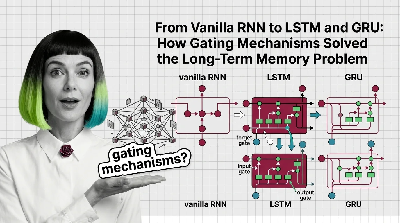
Table of Contents
ELI5
A vanilla RNN forgets long sequences because gradients shrink to near zero. Gating mechanisms (LSTM and GRU) add learnable switches that decide what to remember, what to forget, and what to output.
Here is a pattern that should bother you: a Recurrent Neural Network trained on English text can predict the next word in a five-word clause with reasonable accuracy — then collapse into incoherence when the relevant context sits forty tokens back. The network didn’t run out of capacity. It ran out of gradient signal. The information was there at timestep one; by timestep forty, the math had quietly erased it.
That failure — and the specific mechanism behind it — is what makes gating architectures worth understanding, not as incremental improvements but as a fundamentally different answer to the question of how a network should handle time.
The Gradient Cliff: Why Vanilla RNNs Forget
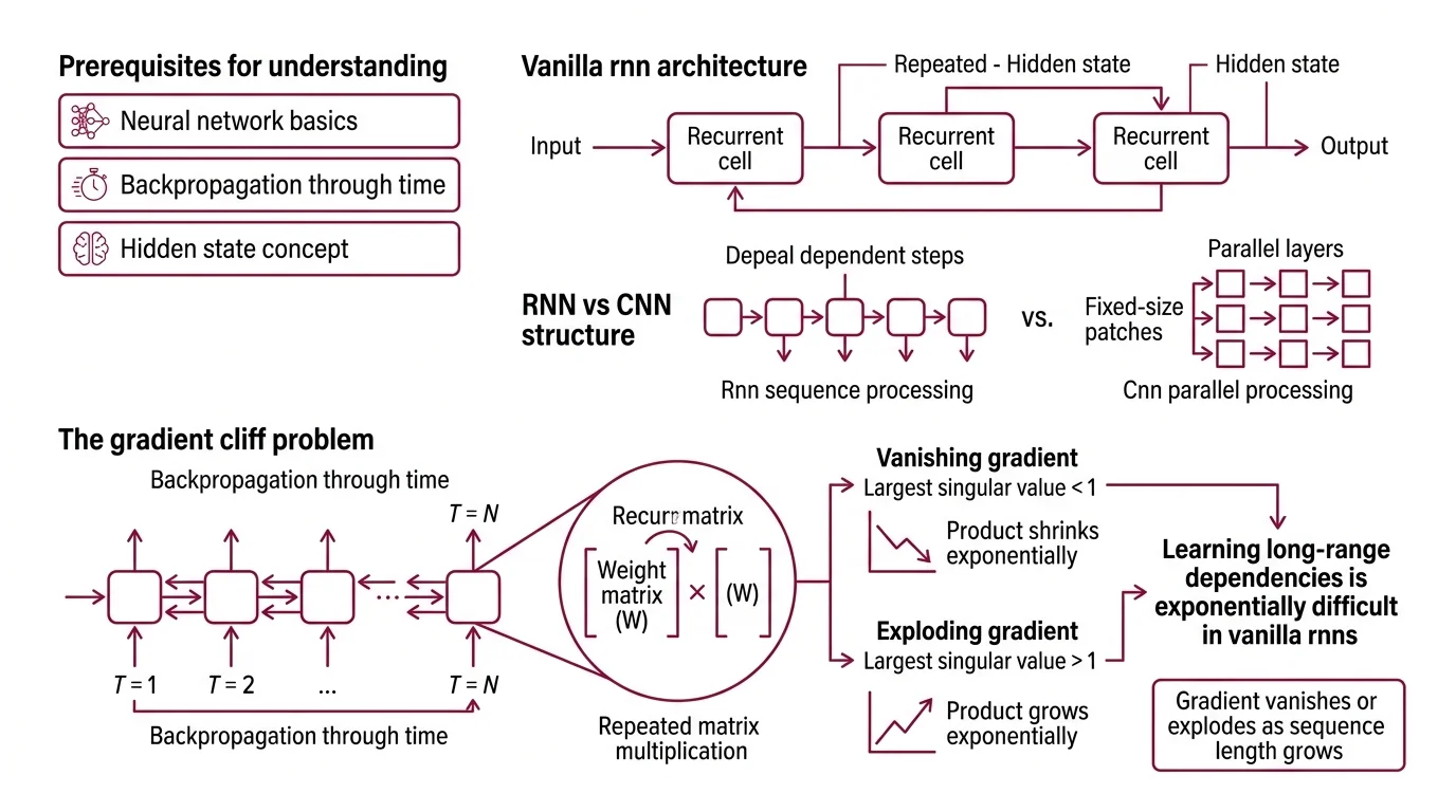
The original recurrent architecture, proposed by Elman (1990), had a clean elegance: feed the output of one timestep back into the input of the next. A single weight matrix, applied recursively, creates a chain of dependencies across time. In principle, this chain can carry information from the first token to the last.
In practice, the chain breaks.
What math and neural network concepts do you need before learning RNNs and LSTMs?
To follow the mechanism, you need three prerequisites. First, Neural Network Basics for LLMs — the concept of layers, weights, and activation functions that transform inputs into outputs. Second, Backpropagation Through Time — the algorithm that unrolls the recurrence and computes gradients across timesteps, which is where the failure originates. Third, a working sense of how a Hidden State carries compressed information forward through a sequence, acting as the network’s only channel for temporal context.
You should also understand how a Convolutional Neural Network extracts spatial features, because the contrast is instructive: CNNs process fixed-size patches in parallel, while RNNs process tokens sequentially, creating a dependency chain whose length directly determines gradient stability.
The mathematical root of the problem is repeated matrix multiplication. During backpropagation through time, the gradient of the loss with respect to early timesteps involves multiplying the recurrent weight matrix by itself once per timestep. If the largest singular value of that matrix is less than one, the product shrinks exponentially. If greater than one, it explodes. Bengio et al. (1994) formalized this: learning long-range dependencies via gradient descent is exponentially difficult in vanilla RNNs because the gradient either vanishes or explodes as the sequence length grows.
The vanishing case is worse, practically speaking. Exploding gradients announce themselves — the loss spikes, the weights overflow, training crashes. Vanishing gradients are silent. The network trains, the loss decreases, the outputs look plausible. But the model has quietly abandoned any attempt to connect distant tokens. It learns local patterns and ignores everything else.
Selective Memory: The LSTM Architecture
Hochreiter and Schmidhuber proposed the Long Short-Term Memory network in 1997 to solve this problem — not by fixing gradient flow through the recurrent weight matrix, but by building a parallel highway that gradients could traverse without repeated multiplication.
The key insight is a dedicated cell state: a vector that runs through the entire sequence with only additive and element-wise multiplicative operations. Gradients flowing along this cell state encounter addition, not matrix multiplication, which means they neither vanish nor explode by default. The cell state is the architectural solution to the gradient cliff.
But an unregulated highway is useless. If everything gets added and nothing gets removed, the cell state saturates with noise. This is where gating enters.
How do LSTM forget gates, input gates, and output gates control information flow?
Three learned gates regulate what enters, persists in, and exits the cell state — each is a sigmoid layer that outputs values between zero and one, element-wise.
The forget gate reads the current input and the previous hidden state, then produces a mask: values near one preserve the corresponding cell state element; values near zero erase it. This is the mechanism by which the network learns to discard information that is no longer relevant — a closed parenthesis can signal that the clause-level context should be cleared.
The input gate controls what new information gets written. It works in tandem with a candidate layer (typically a tanh activation) that proposes new values. The gate selects which candidates actually reach the cell state. Without this gate, every timestep would overwrite the cell with fresh data, destroying long-range memory.
The output gate determines which parts of the cell state are exposed as the hidden state for the current timestep. The cell might store information needed five steps from now but irrelevant to the immediate next-token prediction — the output gate keeps it hidden until it matters.
The result is a network that can, in principle, carry a signal across hundreds of timesteps without degradation. The cell state is a protected memory line; the gates are learned read-write-erase heads. Not a metaphor. A functional description: the forget gate erases, the input gate writes, the output gate reads.
The Architectural Fork: LSTM Versus GRU
LSTM proved that gating could rescue recurrence from gradient death. The next question was architectural economy: how many gates does the job actually require? The answer split the field into two competing designs with different trade-offs but surprisingly similar results.
What is the difference between vanilla RNN, LSTM, and GRU architecture?
The vanilla RNN has one recurrence equation, one weight matrix, and no gating. Every timestep overwrites the hidden state with a new combination of input and previous state, passed through a single activation function. There is no mechanism to protect information from being overwritten or to selectively forget.
LSTM adds a cell state and three gates — six weight matrices where the vanilla RNN had one. This solves the vanishing gradient problem but introduces substantial parameter overhead. For a hidden dimension of 512, an LSTM layer has roughly four times the parameters of the equivalent vanilla RNN layer.
The Gated Recurrent Unit, introduced by Cho et al. (2014), asked a practical question: does the LSTM need all three gates?
GRU collapses the forget and input gates into a single update gate — a value near one means “keep the old state,” a value near zero means “replace it with new information.” There is no separate cell state; the hidden state itself serves both roles. A reset gate controls how much of the previous hidden state influences the candidate for the new state, providing a mechanism for the network to act as if it were starting fresh when the sequence context demands it.
| Property | Vanilla RNN | LSTM | GRU |
|---|---|---|---|
| Gates | 0 | 3 (forget, input, output) | 2 (update, reset) |
| Cell state | No | Yes (separate from hidden state) | No (hidden state only) |
| Gradient protection | None | Additive cell state highway | Additive hidden state updates |
| Parameter count (relative) | 1x | ~4x | ~3x |
| Long-range dependency handling | Poor | Strong | Strong |
The performance comparison is instructive in its ambiguity. Empirical evaluations found similar accuracy on polyphonic music modeling, speech signal modeling, and standard NLP benchmarks (Wikipedia). Neither architecture consistently dominates. The difference is computational, not representational — GRU trains faster and uses less memory, LSTM offers finer-grained control over what gets stored versus exposed.
What the Gate Equations Predict in Practice
The gating framework turns passive understanding into diagnostic intuition. If an LSTM-based model fails on a task that requires tracking a specific entity across a long passage, the failure mode is almost always the forget gate: it learned to erase the entity’s representation before the model needed it. If the model generates text that ignores recent context — repeating a pattern established early in the sequence — the input gate is likely too conservative, preventing recent information from overwriting stale cell state values.
For GRU-based models, the diagnostic is simpler but coarser. The update gate controls the tradeoff between persistence and novelty in a single parameter. If a GRU model oscillates between two behaviors depending on sequence length, the update gate’s learned bias is the first place to look.
Rule of thumb: Choose LSTM when the task requires the model to store information it doesn’t immediately use (the output gate provides this capability). Choose GRU when training speed matters and the task doesn’t require latent storage — translation, short-sequence classification, speech recognition on fixed-length utterances.
When it breaks: Both architectures process sequences token by token, creating an inherent bottleneck: training time scales linearly with sequence length, and parallelization across timesteps is impossible. For sequences beyond a few thousand tokens, this sequential dependency makes LSTMs and GRUs impractical compared to attention-based architectures that process all positions simultaneously. The gating mechanism solved the gradient problem but not the throughput problem — which is why Transformers, despite their quadratic memory cost, displaced recurrent architectures for most large-scale language tasks.
A coda: the LSTM is not a closed chapter. Beck et al. (2024) introduced xLSTM at NeurIPS 2024, replacing the sigmoid gates with exponential gating and adding a matrix-valued memory cell (mLSTM) that is fully parallelizable. The xLSTM 7B model, trained on 2.3 trillion tokens and released as open weights (NXAI Blog), reopens the question of whether recurrence itself was the bottleneck — or only the specific form of recurrence we abandoned.
The Data Says
The vanishing gradient problem was not a limitation of the recurrence idea — it was a limitation of unregulated recurrence. LSTM’s cell state highway and GRU’s update gate both solve it by replacing repeated matrix multiplication with additive updates, protecting gradient signal across hundreds of timesteps. The architectural question that remains open is whether parallelizable recurrence, as in xLSTM, can match Transformer throughput without surrendering the gating intuition that made long-range memory tractable in the first place.
AI-assisted content, human-reviewed. Images AI-generated. Editorial Standards · Our Editors