From True Positives to Macro Averaging: The Building Blocks Behind Precision, Recall, and F1

A classifier that labels every email as “not spam” will score 99.5% accuracy — if only 0.5% of your inbox is junk. It never catches a single phishing attempt, never flags a single scam, and by the most widely reported metric in machine learning, it looks nearly perfect. This is the gap that Precision, Recall, and F1 Score exists to close: the distance between a number that sounds right and a measurement that tells you where your model actually fails.

The Arithmetic of Getting It Wrong

Every classification decision lands in one of four bins. The names sound deceptively simple — true positive, false negative — until you realize they encode a geometry of errors, and that geometry is what separates a model that “works” from one you can trust.

What are true positives, false positives, and false negatives in classification?

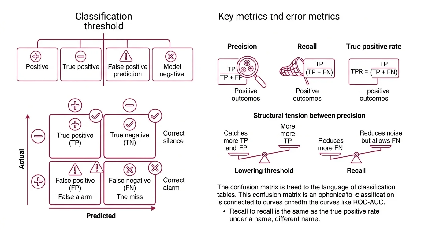
A Classification Threshold divides your model’s continuous output into positive and negative predictions. From that boundary, four outcomes emerge:

• True positive (TP): the model predicted positive, and the sample is positive. The correct alarm.
• True negative (TN): the model predicted negative, and the sample is negative. The correct silence.
• False positive (FP): the model predicted positive, but the sample is negative. The false alarm.
• False negative (FN): the model predicted negative, but the sample is positive. The miss.

Precision is TP / (TP + FP) — of everything you called positive, what fraction actually was? Recall is TP / (TP + FN) — of everything that was actually positive, what fraction did you catch? These two ratios are the questions that raw accuracy compresses into silence.

The tension between them is structural. Lowering the threshold catches more true positives but drags in more false alarms; raising it reduces noise but lets real positives slip through. Precision and recall move in opposition unless the model itself improves — and recognizing that constraint is the first step toward choosing which errors you can afford.

The True Positive Rate, which is recall under a different name, connects this vocabulary directly to Roc Auc analysis. Same numerator, same denominator, different framing — one speaks the language of classification tables, the other speaks the language of curves.

What is a confusion matrix and how do you read it for multiclass problems?

A Confusion Matrix is the full ledger. For binary problems it is a 2x2 grid: true labels on the rows, predicted labels on the columns. Each cell holds a count. The diagonal contains your correct answers; everything off-diagonal is a specific type of mistake.

In Scikit Learn, the convention is explicit: C[i, j] represents the number of observations with true label i that the model predicted as label j (scikit-learn Docs). Rows are ground truth. Columns are predictions.

For multiclass problems the matrix expands to NxN, and here it transforms from a summary statistic into a diagnostic map. Suppose your sentiment classifier consistently predicts “neutral” when the true label is “negative.” That pattern appears as a bright spot in a specific off-diagonal cell — row “negative,” column “neutral.” You do not just know the model is wrong; you know the direction of the error, and direction is what tells you where to intervene.

Reading a multiclass confusion matrix is less about the aggregate count and more about the asymmetries. Which classes does the model confuse with each other? Where is the diagonal weakest? Those cells are your engineering targets — not the overall accuracy number printed at the top of the notebook.

Three Ways to Average the Same Number

F1 is the harmonic mean of precision and recall: F1 = 2 * (precision * recall) / (precision + recall), equivalently 2TP / (2TP + FP + FN) (Wikipedia, F-score). The harmonic mean punishes imbalance — if either precision or recall drops toward zero, F1 follows hard. That is the point. A model with excellent precision but terrible recall cannot hide behind an arithmetic average.

But F1 is defined for a single class. When your problem has five classes, or ten, or a thousand, a different question surfaces: how do you aggregate per-class scores into one number?

What is the difference between micro, macro, and weighted F1 score?

Three strategies exist. They answer three different questions about performance, and choosing the wrong one can make a failing model look acceptable.

Macro F1 computes F1 independently for each class, then takes the arithmetic mean. Every class gets equal weight regardless of how many samples it contains (scikit-learn Docs). A rare disease class with fifty samples and a healthy class with fifty thousand contribute identically. Macro F1 is the metric that forces your model to care about minorities — and it is the one that reveals failures that other averages bury.

Micro F1 pools all true positives, false positives, and false negatives across classes before computing a single F1. In single-label classification, a consequence: micro precision, micro recall, and micro F1 all collapse to the same number — plain accuracy (scikit-learn Docs). Micro F1 tells you how the model performs on the average sample, not the average class.

Not the same question. Not even close.

Weighted F1 computes per-class F1 and averages by support — the number of true instances in each class (scikit-learn Docs). It is the middle ground: rare classes still contribute, but proportionally to their prevalence in the dataset.

The choice between them is not mathematical. It is a decision about what failure you refuse to tolerate. In fraud detection, where Class Imbalance is extreme and missing the rare class is catastrophic, macro F1 exposes weaknesses that micro F1 buries. In balanced multiclass tasks, the three variants converge — and the distinction barely matters. The metric does not change. Your context does.

When Rank Matters More Than Count

Classification metrics count hits and misses across every prediction. But some systems — search engines, recommendation engines, retrieval-augmented generation pipelines — care about something different: where in the ranked list the relevant items appear.

What are precision at k and recall at k in information retrieval?

Precision@K and Recall@K migrate the precision/recall vocabulary from classification into ranked retrieval, but the semantics shift in ways that matter.

Precision@K = (relevant items in the top K results) / K (Evidently AI). Of the K items you showed the user, what fraction was relevant? If a search engine returns ten results and three are useful, Precision@10 is 0.3.

Recall@K = (relevant items in the top K results) / (total relevant items in the dataset) (Evidently AI). Of all the relevant items that exist anywhere in the corpus, what fraction surfaced in your top K? If the dataset contains twenty relevant documents and your top ten includes six, Recall@10 is 0.3.

The distinction from classification precision and recall is structural. In classification, every sample receives a prediction. In retrieval, only the top K items are evaluated — and K is a design choice, not a property of the data. A system with poor Precision@5 might have strong Precision@50, depending on how relevant items distribute across ranks.

This connects to Model Evaluation more broadly. A retrieval system’s quality depends on where you draw the cutoff. A classifier’s quality depends on the threshold you set. Both are decisions about drawing a line between “included” and “ignored” — and both force the same underlying trade-off between catching more relevant items and being wrong about fewer of them.

What the Formulas Predict

If you shift the classification threshold lower, recall rises but precision drops — mechanically, inevitably, unless the model’s underlying separability improves. If macro F1 is high but micro F1 is low, a majority class is dragging down the pooled counts. If the reverse is true, a minority class is failing badly and the macro average is broadcasting that failure while micro F1 hides it.

These are not rules of thumb. They are consequences of the arithmetic.

In practice:

• If two classes occupy overlapping regions in feature space, the confusion matrix will show symmetric off-diagonal errors between them. Better features or a finer decision boundary fix this — a different metric does not.
• If Precision@K is low but Recall@K is acceptable, your ranking algorithm buries relevant items too deep. The items exist; they are not surfacing early enough.
• If recall is high but precision is low, you are flooding downstream systems with false positives. In spam filtering, that means legitimate emails in the junk folder. In medical screening, that means unnecessary procedures.

Rule of thumb: Choose the metric that penalizes the failure mode your application cannot afford.

When it breaks: F1 assumes precision and recall are equally important. When they are not — when a missed cancer diagnosis costs orders of magnitude more than a false alarm — F1 is the wrong target. The F-beta score weights recall higher when beta > 1 and precision higher when beta < 1, letting you encode that asymmetry directly into the metric. And when Benchmark Contamination is present, all metrics become unreliable regardless of averaging strategy, because the model’s apparent performance reflects memorization rather than generalization.

The Data Says

Precision, recall, and F1 are not interchangeable views of the same truth — they are different questions about different failure modes. The confusion matrix is the diagnostic; the averaging strategy is the lens that determines what failures you see through it. Collapsing them into a single number always requires a decision about which errors matter most, and that decision belongs to the engineer who understands the consequences, not the one who understands the math.