From ReLU to SwiGLU: How Activation and Loss Functions Shape LLM Training
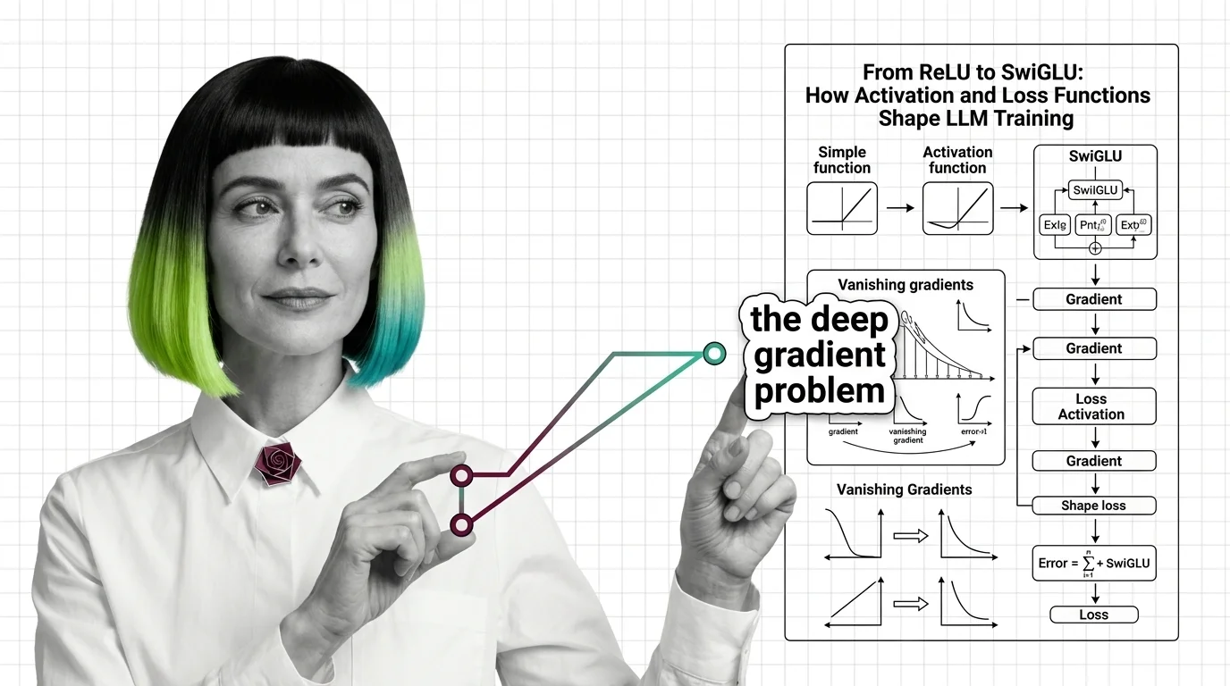
Table of Contents
ELI5
Activation and loss functions control what a model learns during training. Activations gate which signals pass between layers. Loss measures prediction error and sends corrections backward. Together, they determine every weight update the model makes.
Same architecture. Same data. Same compute budget. Change one function — the Activation Function in the feed-forward block — and training quality shifts measurably. ReLU’s formula fits on a napkin. SwiGLU’s barely fills a paragraph. Yet the dominant open-weight models released after 2023 — LLaMA, Mistral, Gemma, DeepSeek — all chose SwiGLU, and the paper that introduced it offered no theoretical explanation for why it outperforms the alternatives (Shazeer, 2020). That gap between empirical result and missing theory is exactly the kind of anomaly worth tracing to its source.
The Gate That Decides What Gets Through
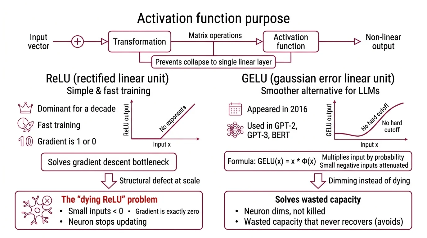
Every layer in a Neural Network Basics for LLMs receives a vector of numbers — activations from the previous layer — and must decide what to pass forward. Without an activation function, the entire network collapses into a single linear transformation, regardless of how many layers you stack. Multiplying matrices by matrices still yields a matrix. The activation function is what breaks that linearity and gives depth its purpose.
What activation functions are used in large language models
ReLU — Rectified Linear Unit — dominated deep learning for roughly a decade. Its formula is almost insulting in its simplicity: output the input if it is positive, output zero otherwise. No exponents, no probability distributions, no learned parameters. It trains fast because the gradient is either 1 or 0, and it solved the Gradient Descent bottleneck that had stalled deeper networks through the 2000s.
But ReLU carries a structural defect that becomes expensive at scale.
When an input falls below zero, the gradient is exactly zero — permanently. The neuron stops updating. In a small network, a few dead neurons are a rounding error. In a model with billions of parameters, dead neurons represent wasted capacity that never recovers. This is the “dying ReLU” problem (Ultralytics Glossary), and it is the pressure that drove the search for smoother alternatives.
GELU — Gaussian Error Linear Unit — appeared in 2016. Instead of a hard cutoff at zero, GELU multiplies the input by the probability that a standard Gaussian random variable would fall below that value: GELU(x) = x * Φ(x), where Φ is the standard Gaussian CDF (Hendrycks & Gimpel, 2016). The effect is that small negative inputs get attenuated rather than killed outright. The neuron dims instead of dying. GPT-2, GPT-3, and BERT all used GELU in their feed-forward layers — it became the default activation for the 2018-2022 generation of transformers.
Then came SwiGLU, and the architecture of the feed-forward block itself changed.
Noam Shazeer proposed SwiGLU in “GLU Variants Improve Transformer” (Shazeer, 2020). The difference is not just the nonlinearity — it is structural. Instead of one weight matrix transforming the input before an activation, SwiGLU uses a gated mechanism with two parallel linear projections: SwiGLU(x, W, V) = Swish(xW) ⊗ (xV), where ⊗ is element-wise multiplication and Swish is what PyTorch implements as SiLU. Three weight matrices per feed-forward layer instead of two. Roughly 50% more parameters per layer — but consistently better training quality on downstream tasks.
SwiGLU and GEGLU produced the best perplexities compared to ReLU and GELU baselines in experiments on T5 (Shazeer, 2020). LLaMA 2 and 3, Mistral, Mixtral, Gemma, PaLM, and DeepSeek all adopted SwiGLU (NVIDIA Docs). In the post-2023 wave of open-weight LLMs, SwiGLU became the default.
The theoretical justification for SwiGLU’s advantage remains incomplete. The empirical gain is reproducible across architectures and scales. The mechanism behind it is not fully characterized — which is either humbling or reassuring, depending on how much certainty you require before trusting your infrastructure.
One Number That Measures How Wrong You Are
A Loss Function takes the model’s prediction and the correct answer and returns a single number — the distance between them. That number is the error signal. Everything the model learns during training, it learns by making that number smaller through Backpropagation.
What is cross-entropy loss and how does it train language models
For next-token prediction — the training objective of autoregressive LLMs — the standard loss is Cross Entropy Loss. The formula is deceptively compact: L = -log(p_y), where p_y is the probability the model assigned to the correct next token (PyTorch Docs).
Think of the model’s output as a probability distribution stretched across the entire vocabulary — tens of thousands of possible tokens. Cross-entropy measures how far this predicted distribution sits from the ideal one, where the correct token has probability 1 and everything else has probability 0. The asymmetry is sharp — confident wrong answers cost exponentially more; assigning probability 0.01 to the correct token produces a much larger gradient than assigning 0.3.
Not a quirk. The mechanism.
That asymmetry means the model learns fastest precisely when it is most wrong. As predictions improve, the gradient diminishes and the model shifts from overhauling its representations to fine-tuning them. This is why training loss curves are steep early and shallow late — the loss function itself throttles the learning rate implicitly, independent of any optimizer schedule.
But there is a catch. The gradient that cross-entropy generates must travel backward through every layer of the network — dozens of them, sometimes over a hundred. And that journey has a failure mode that nearly killed deep learning before it began.
When the Gradient Disappears
Deep networks learn by passing error gradients backward from the output layer through every intermediate layer to the first. At each layer, the gradient is multiplied by the local derivative of that layer’s activation function. If those local derivatives are consistently less than 1, the gradient shrinks exponentially with depth. If they are consistently greater than 1, the gradient explodes.
Why do deep neural networks suffer from vanishing and exploding gradients
Sepp Hochreiter identified the vanishing gradient problem in his 1991 diploma thesis at TU Munich (Wikipedia). The arithmetic is blunt: a gradient passing through 100 layers, each multiplying by 0.9, arrives at the first layer scaled by 0.9 to the 100th power — roughly 0.00003. The early layers receive a learning signal so attenuated they barely update their weights. The network has depth on paper but learns as if its first layers were frozen in place.
Exploding gradients are the mirror failure. Local derivatives above 1, compounded over depth, produce gradients so large that weight updates overshoot and destabilize training. The model does not learn slowly — it destroys what it already learned.
I’ve watched training runs collapse in exactly this way: loss drops steadily for hours, then a single batch produces a gradient spike that sends the weights into a region from which the model never recovers. The loss curve doesn’t plateau. It detonates.
Three innovations, arriving within a five-year window, made modern depth possible: ReLU in 2010, batch normalization in 2015, and residual connections in 2015 (Wikipedia). ReLU addressed vanishing gradients because its derivative is exactly 1 for positive inputs — no shrinkage. Batch normalization stabilized the distribution of intermediate activations so layers stopped chasing moving targets. Residual connections created a gradient highway — a skip path that lets the error signal flow directly across layers without being multiplied down at each step.
Modern LLMs combine all three strategies, though the specific activation function has since evolved from ReLU through GELU to SwiGLU. The vanishing gradient problem is managed, not eliminated — and that distinction shapes every architectural decision, from layer count to learning rate scheduling to the choice of optimizer.
What the Functions Predict About Your Training Run
The choice of activation function is not cosmetic. Switching from GELU to SwiGLU in a feed-forward block adds roughly 50% more parameters per layer — a concrete cost in memory and compute. The tradeoff is better gradient flow through the gated structure and, empirically, lower perplexity. For smaller models where parameter budget is tight, that overhead may not justify itself. For large-scale training runs where quality per compute dollar matters, the post-2023 consensus is clear.
Cross-entropy loss creates a specific training dynamic: the model learns fastest from its worst predictions and decelerates as it improves. If you see training loss plateau early, the gradient signal has likely weakened below the threshold where the optimizer can make progress — a sign to examine learning rate warmup, data mixing, or whether model capacity matches task complexity.
If training loss drops steeply but validation loss stalls, the loss function is doing its job — the model is overfitting, not underlearning. The fix lives in the data or regularization strategy, not in the loss function.
Rule of thumb: activation function choice determines the quality of forward signal propagation; loss function choice determines the quality of backward error propagation. Neither decision is independent of the other — they co-determine the gradient geometry of the optimization.
When it breaks: SwiGLU’s extra parameter cost becomes a liability when memory is the binding constraint. On edge devices or with very long context windows, the 50% parameter overhead per feed-forward layer can force tradeoffs between model depth and sequence length. The activation function that helps at scale can hurt at the margins.
The Data Says
Activation functions and loss functions are not accessories bolted onto the architecture. They are the mechanisms that determine whether depth produces learning or produces noise. The evolution from ReLU to SwiGLU traces a single engineering arc: keep the gradient alive, let the gate decide what passes through, and accept the parameter cost. Cross-entropy loss converts prediction error into a learning signal whose strength is proportional to the model’s confidence in the wrong answer. Every architectural choice in a modern LLM — layer count, normalization, residual connections — exists to protect that signal on its journey backward through depth.
AI-assisted content, human-reviewed. Images AI-generated. Editorial Standards · Our Editors