From LeNet to ConvNeXt: How CNN Architectures Evolved and Where Spatial Inductive Bias Falls Short
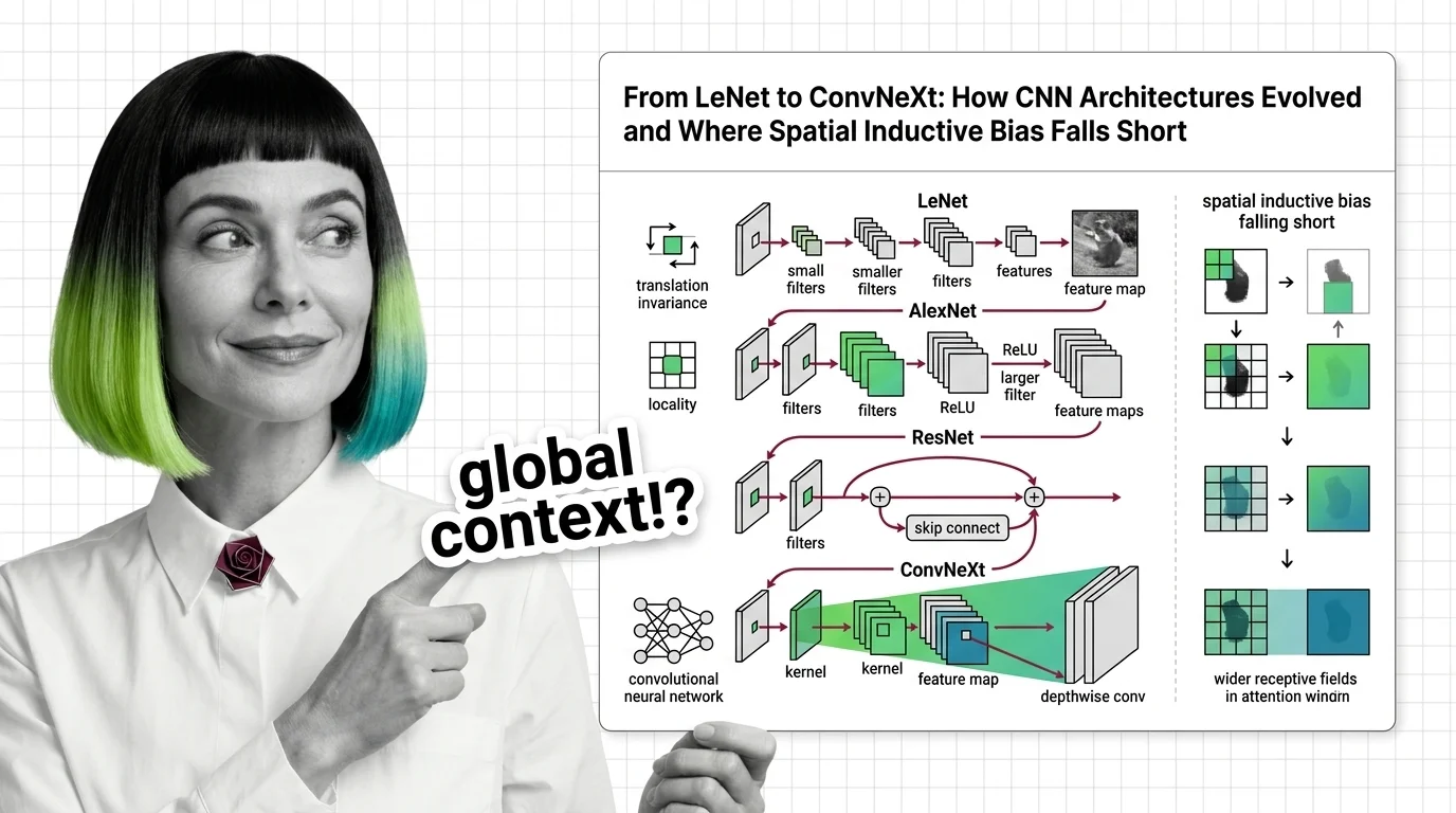
Table of Contents
ELI5
A convolutional neural network slides small filters across an image to detect patterns — edges first, then shapes, then objects. This spatial awareness makes CNNs efficient, but it also means they struggle to see the full picture at once.
In 2012, a neural network with eight layers cut image classification error nearly in half — then couldn’t be made meaningfully deeper without accuracy collapsing. Three years later, a 152-layer network trained stably; not because someone added more compute, but because someone added a shortcut. The history of Convolutional Neural Network architectures is less a story about stacking layers and more about discovering which constraints to keep and which to throw away.
The Vocabulary Before the Convolution
Every architectural leap in CNN history builds on a small set of mathematical and computational ideas. Skip them, and the papers read like incantations. Understand them, and the design choices become almost obvious.
What math and neural network concepts do you need before learning convolutional neural networks?
Start with linear algebra — specifically matrix multiplication and element-wise operations, because convolution is a structured form of both. A convolutional layer applies a small weight matrix (the kernel) across spatial positions of the input, producing a Feature Map that encodes where a pattern was detected and how strongly.
That operation relies on three ideas from Neural Network Basics for LLMs: the forward pass (input times weights yields output), backpropagation (computing gradients to update those weights), and nonlinear activation functions (without which stacking layers would collapse into a single linear transformation). You also need to understand what a loss function measures and why gradient descent moves weights toward lower loss — because every architectural innovation in this article is, at bottom, an answer to the question of why gradients sometimes stop flowing.
Partial derivatives and the chain rule matter more here than in most ML subfields, because CNN depth amplifies gradient behavior. When gradients shrink exponentially across layers (the vanishing gradient problem), deep networks stop learning. When they grow exponentially (the exploding gradient problem), training destabilizes. The entire arc from LeNet to ResNet is a series of engineering responses to this single mathematical reality.
Probability theory and basic statistics help with understanding batch normalization and dropout — regularization techniques that became standard after AlexNet. But the core prerequisite is geometric: if you can visualize a small matrix sliding across a larger one and producing a third, you have the mental model that makes everything else click.
Four Leaps That Changed What Depth Means
The distance between LeNet and ConvNeXt is not measured in parameters alone — it is measured in how each architecture answered a recurring question: how do you make a network deeper without breaking the gradient signal?
How did CNN architectures evolve from LeNet to AlexNet to ResNet to ConvNeXt?
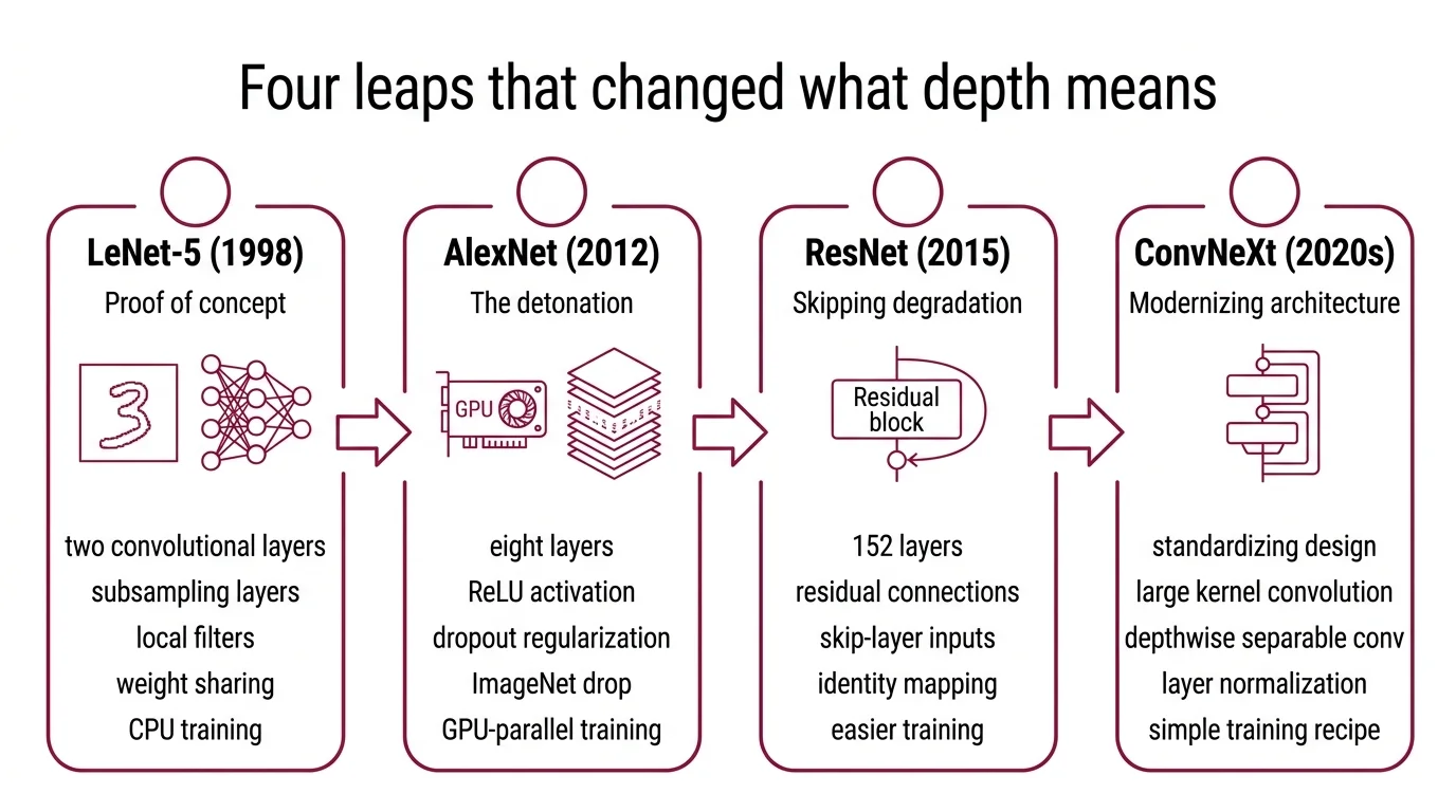
LeNet-5 (1998) was the proof of concept. Yann LeCun and colleagues built a network with two convolutional layers, two subsampling layers, and two fully connected layers — roughly 60,000 parameters trained on 32x32 grayscale images of handwritten digits (LeCun et al.). The architecture was small enough to train on a single CPU, and it worked. But the insight that mattered was not the accuracy; it was the principle that learned local filters could replace hand-engineered feature extractors. LeNet showed that spatial structure in the input — neighboring pixels correlate — could be exploited by the architecture itself, through weight sharing and local connectivity.
For more than a decade, that principle waited.
AlexNet (2012) was the detonation. Krizhevsky, Sutskever, and Hinton entered the ImageNet Large Scale Visual Recognition Challenge and dropped the top-5 error rate from 26% to 15.3% — a gap so wide it ended the debate over whether deep learning could outperform traditional computer vision pipelines (Wikipedia, AlexNet). AlexNet scaled to eight layers (five convolutional, three fully connected), replaced sigmoid activations with ReLU (which does not saturate for positive inputs, easing gradient flow), introduced dropout as regularization, and — critically — trained on GPUs. The architectural vocabulary of modern CNNs starts here: ReLU, dropout, GPU-parallel training, and the confidence that bigger networks could mean better performance.
But AlexNet also exposed a ceiling. Making the network substantially deeper did not automatically improve results; gradients degraded across too many layers, and training became unstable.
ResNet (2015) broke through that ceiling with a structural shortcut. He, Zhang, Ren, and Sun introduced Residual Connections: instead of requiring each layer to learn the full mapping from input to output, they added skip connections that let the input bypass one or more layers. The network only needed to learn the residual — the difference between input and desired output. This seemingly minor change made networks of 152 layers trainable and achieved 3.57% top-5 error on ImageNet, winning the 2015 ILSVRC across classification, detection, and localization (He et al.).
The mathematical reason residual connections work is elegant: they provide a gradient highway. During backpropagation, the skip connection carries the gradient signal directly to earlier layers, bypassing the multiplicative chain that causes vanishing gradients. Depth stopped being a liability and became a design parameter.
ConvNeXt (2022) asked an uncomfortable question: what if the transformer’s advantage was partly configuration, not architecture? Liu and colleagues started with a standard ResNet-50 and systematically modernized it toward the design choices used in Swin Transformer: a patchify stem (replacing the traditional stride-4 convolution), 7x7 depthwise separable convolutions, inverted bottleneck blocks, GELU activation, and LayerNorm instead of BatchNorm (HuggingFace Course). The result — ConvNeXt V1 — reached 82.0% top-1 accuracy on ImageNet-1K, surpassing Swin Transformer’s 81.3% (HuggingFace Course).
ConvNeXt V2, published at CVPR 2023, pushed further with a fully convolutional masked autoencoder framework (FCMAE) and a Global Response Normalization layer. The Huge model — 650 million parameters — reached 88.9% top-1 accuracy on ImageNet, trained with ImageNet-22K pre-training followed by ImageNet-1K fine-tuning (ConvNeXt V2 paper).
Not a paradigm shift. A controlled experiment.
The Blind Spot in Every Kernel
Local receptive fields are the CNN’s greatest strength and its most fundamental constraint. Every convolutional kernel sees only a small neighborhood of pixels; deeper layers combine these local views into increasingly abstract representations. But some patterns in visual data are inherently non-local — and no amount of stacking can fully compensate.
Why do CNNs struggle with global context and long-range dependencies compared to vision transformers?
The core issue is receptive field growth versus computational cost. A 3x3 kernel at layer one sees nine pixels. After many stacked layers, the theoretical receptive field can span the entire image — but the effective receptive field (the region that meaningfully influences the output) is typically much smaller, concentrated near the center. Long-range dependencies — a shadow relating to an object across the image, a background cue that disambiguates a foreground object — require the network to integrate information across spatial positions that the architecture treats as distant.
Vision Transformers take a different approach entirely. The ViT architecture, introduced by Dosovitskiy and colleagues at ICLR 2021, splits an image into 16x16 patches and processes them as a sequence with self-attention — a mechanism where every patch attends to every other patch from the first layer (Dosovitskiy et al.). There is no concept of locality built into the architecture. Global context is available immediately, not earned through depth.
This difference has a mathematical name: inductive bias. CNNs encode a strong spatial prior — translation equivariance — which means the network treats a pattern the same way regardless of where it appears in the image. That prior is extremely useful; it is why CNNs learn efficiently with limited data. But it is also a constraint: the network assumes spatial locality matters, and it cannot easily override that assumption for tasks where it does not.
ViT lacks this spatial prior, which is why it requires large-scale pre-training — the original architecture needed datasets of 100 million or more images to outperform CNNs on standard benchmarks (Dosovitskiy et al.). Without the locality constraint, the model has more freedom but also more parameters to tune, and small datasets do not provide enough signal.
The emerging response to this tension is hybrid architectures that combine convolutional spatial priors with transformer-style global attention. ConvNeXt itself hints at this direction: by borrowing design patterns from transformers (larger kernels, LayerNorm, inverted bottlenecks), it narrowed the accuracy gap — suggesting that part of what made transformers effective was not self-attention per se, but the engineering decisions surrounding it.
Where the Gradient Runs Out and the Context Falls Short
The practical consequences of this architectural history are concrete enough to guide design decisions.
If you are building a vision system with limited labeled data, CNNs remain the more sample-efficient choice — their spatial inductive bias provides structure that the network would otherwise have to learn from scratch. If your task requires understanding global relationships within the image (document layout analysis, scene-graph prediction, long-range object interactions), the effective receptive field of a deep CNN may not reach far enough, and a transformer-based or hybrid approach will likely outperform it.
Rule of thumb: Use CNN backbones when data is scarce and spatial locality is a strong prior for the task; switch to transformers or hybrids when the task demands global context and you have sufficient data to compensate for the weaker inductive bias.
When it breaks: CNNs fail predictably when the discriminative signal lies in relationships between distant image regions — where the effective receptive field, no matter how many layers you add, does not meaningfully cover the spatial extent of the relevant pattern.
Compatibility note:
- timm library: The legacy import path
timm.models.layersis deprecated; usetimm.layersinstead when working with ConvNeXt implementations.
The Data Says
CNN architectures did not evolve by getting deeper. They evolved by solving the same problem in increasingly precise ways: how to preserve gradient signal across depth while extracting useful spatial features. ConvNeXt demonstrated that much of the transformer’s apparent advantage was attributable to modernized training and design patterns, not self-attention alone. But the fundamental limitation of local receptive fields remains — convolutions see neighborhoods, not images, and for tasks that demand global context, that constraint is not an implementation detail. It is a boundary in the geometry of the architecture itself.
AI-assisted content, human-reviewed. Images AI-generated. Editorial Standards · Our Editors