From Latent Vectors to Adversarial Loss: The Building Blocks and Prerequisites of GAN Architecture
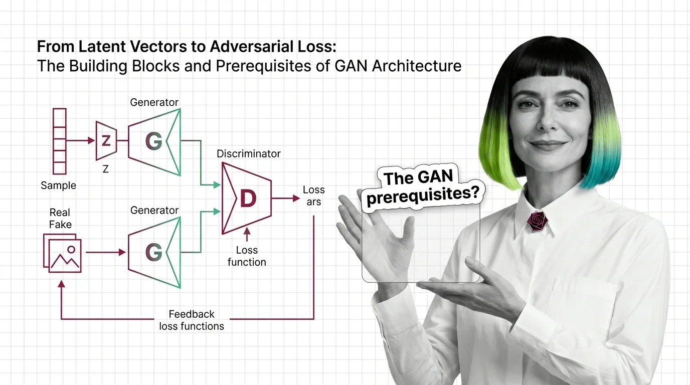
Table of Contents
ELI5
A generative adversarial network pairs two neural networks — one creates fakes, one detects them — and their competition produces increasingly realistic outputs.
Something odd happens when you force two neural networks into opposition. Instead of deadlock, you get synthesis. The generator learns to produce data indistinguishable from the training set — not because it understands what “real” means, but because the discriminator keeps raising the threshold for “convincing.” That adversarial dynamic, formalized by Goodfellow et al. in a 2014 paper that reads more like a game theory proof than a machine learning proposal, is the engine behind every Generative Adversarial Network ever trained.
The Adversarial Engine: Two Networks, One Objective
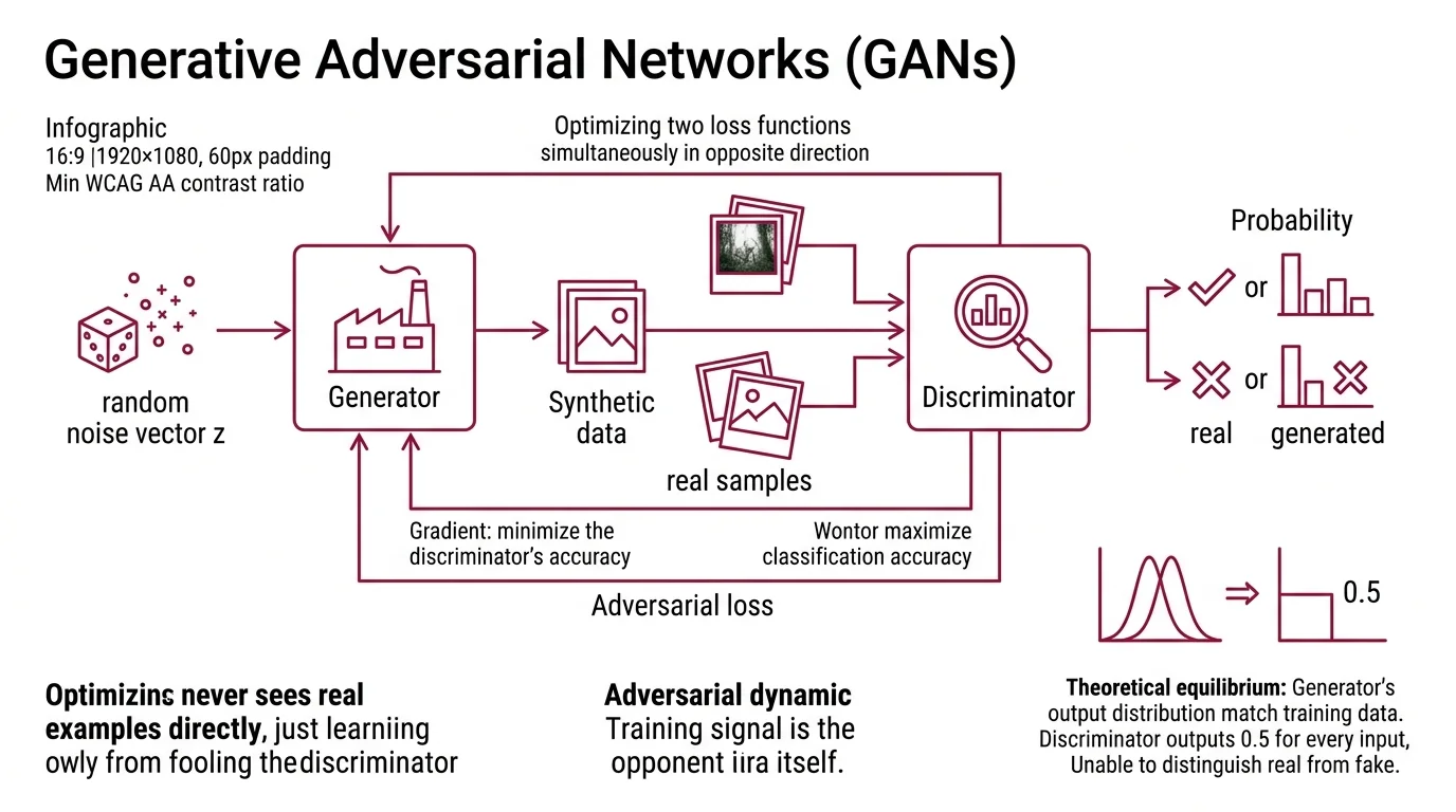
Most architectures optimize a single loss function. GANs optimize two — simultaneously, in opposite directions. The result is a system where neither network has a fixed target; each one’s definition of success shifts as the other improves.
What are the main components of a GAN architecture?
A GAN consists of two Neural Network Basics for LLMs: the generator and the discriminator, locked into what the original paper formalized as a minimax game.
The generator takes a random noise vector z — sampled from a simple distribution like a Gaussian — and maps it through a neural network to produce synthetic data. It never sees real examples directly. Its only learning signal comes from how effectively it fools the discriminator.
The discriminator is a binary classifier. It receives both real samples from the training distribution and fake samples from the generator, then outputs a probability: real or generated (Google Developers). A well-trained discriminator catches subtle statistical signatures that separate authentic data from forgeries — texture inconsistencies, frequency artifacts, distributional gaps that human eyes miss entirely.
The adversarial loss ties them together. The formulation is a minimax objective: the discriminator maximizes its classification accuracy while the generator minimizes it. Formally: min_G max_D E[ln D(x)] + E[ln(1 - D(G(z)))] (Goodfellow et al.). The generator receives gradient information through the discriminator’s judgment — the training signal is the opponent itself, not a labeled dataset of correct outputs. No human annotator decides what “good” looks like. The adversarial dynamic decides.
The theoretical equilibrium is a Nash equilibrium where the generator’s output distribution perfectly matches the training data and the discriminator outputs 0.5 for every input — unable to tell real from fake. At that point, the discriminator is effectively computing the Jensen-Shannon divergence between the two distributions, and it has converged to zero. Proving this equilibrium exists is elegant; reaching it in practice is a different problem — and that gap is where most of the engineering challenge lives.
From Noise to Structure: What the Generator Actually Starts With
A common misunderstanding treats the latent vector as random junk — meaningless noise that the generator somehow sculpts into coherent output. The reality is more geometric and more interesting than that.
What is latent space in a generative adversarial network?
The generator begins each forward pass from a point in Latent Space — a high-dimensional coordinate system where each axis encodes some abstract feature of the output.
Think of a 512-dimensional vector z as a coordinate in a vast space of possibilities. Nearby points produce similar outputs; distant points produce different ones. The generator’s task is learning a function that maps this abstract coordinate system to data space — pixel values, audio waveforms, molecular structures — so that the full distribution of real data is covered.
What makes this space worth studying is its internal geometry. In a well-trained GAN, specific directions in latent space correspond to interpretable attributes: rotate a vector and the generated face turns; move along another axis and hair color shifts. These directions are not programmed into the network. They are geometry learned from adversarial pressure, not assigned by a designer.
Not randomness. Structure.
This is why interpolation between latent points works at all. Walk linearly between two latent vectors and the generated output transitions smoothly between two plausible samples. That continuity is a consequence of the generator learning a smooth mapping — it is not guaranteed by the architecture and breaks down when the latent space is poorly structured or the model is undertrained.
The dimensionality of the latent space is a design choice with direct consequences. Too few dimensions and the generator cannot represent the full data distribution. Too many and the space becomes sparse, making optimization unstable. Most architectures — DCGAN, StyleGAN, Wasserstein GAN — settle on a few hundred dimensions, though the optimal size depends on the complexity of the target domain. The choice shapes how expressive the generator can be, how interpretable the latent space becomes, and how stable training remains throughout the adversarial process.
The Mathematical Bedrock Beneath the Architecture
Every GAN component rests on mathematical machinery that predates adversarial training by decades. The architecture is elegant, but the prerequisites are not optional — skip them and the loss curves become hieroglyphics.
What math and deep learning concepts do you need before learning about GANs?
Four domains form the foundation.
Probability and statistics. GANs are generative models — their entire purpose is learning a probability distribution. You need density functions, expectations, KL divergence, and Jensen-Shannon divergence to read the loss function as more than notation. The minimax objective is an expectation over two distributions; understanding what that expectation represents is the difference between tuning hyperparameters deliberately and guessing.
Calculus and optimization. Backpropagation — the algorithm that propagates error gradients through network layers — is the mechanism by which both networks learn. Gradient descent moves each network’s parameters toward a local optimum, but in a GAN both optimization surfaces shift every step because the opponent is also moving. Standard supervised learning optimizes on a fixed loss surface. GAN training optimizes on one that reshapes itself with every parameter update.
Convolutional Neural Network architectures. The original 2014 paper used fully connected layers, but modern GANs are overwhelmingly convolutional. The DCGAN architecture established the pattern: the generator uses transposed convolutions to upsample latent vectors into images while the discriminator uses standard convolutions to downsample images into classification scores. Understanding how convolutional layers extract spatial hierarchies — edges, textures, compositional patterns — explains why GANs produce the specific artifacts they do and where those artifacts originate in the network.
Recurrent Neural Network concepts matter less for image GANs but become relevant for sequence generation — text, music, time-series data — where the generator must produce ordered outputs with temporal dependencies.
Beyond specific architectures, fluency in neural network fundamentals is non-negotiable: activation functions, batch normalization, learning rate scheduling, and — critically — the difference between a loss that measures classification accuracy and one that measures distributional distance. Adversarial loss measures distributional distance, not accuracy; mistaking the two is one of the most persistent sources of confusion when debugging GAN training.
What the Adversarial Dynamic Predicts — and Where It Fails
If the discriminator is too strong, it provides near-zero gradients to the generator — the vanishing gradient problem. The generator receives no useful signal and stalls. If the discriminator is too weak, the generator produces crude outputs that satisfy a low bar and never refines further. Balance is the central engineering challenge of GAN training, not a secondary tuning concern.
Three failure modes dominate:
- If you train the discriminator significantly more than the generator, expect vanishing gradients — the discriminator’s confidence starves the generator of signal.
- If the generator finds a small subset of outputs that consistently fool the discriminator, expect mode collapse: realistic but repetitive samples that ignore entire regions of the data distribution.
- If the learning rates are mismatched, expect oscillation — the loss curves swing without converging toward equilibrium.
Mode collapse is particularly revealing because it exposes the gap between theory and practice. The minimax proof assumes perfect optimization with infinite capacity and infinite time. Real networks have finite parameters and finite training steps, so the generator often finds local optima that satisfy the adversarial objective while ignoring large parts of the target distribution. The equilibrium exists on paper. Reaching it is an optimization problem that no architecture has fully solved.
As of 2026, diffusion models have largely overtaken GANs for quality-sensitive image generation. But GANs retain a meaningful advantage in real-time inference — roughly two orders of magnitude faster, depending on architecture (Sapien.io) — which keeps them relevant for video filters, game asset generation, and applications where latency matters more than peak fidelity. Hybrid GAN-diffusion architectures are an active research direction, combining adversarial speed with iterative denoising quality.
Compatibility note:
- StyleGAN3 (NVlabs): The official repository is effectively frozen — a one-time code drop with no outside contributions since October 2021. Treat it as a reference implementation, not an actively maintained framework.
Rule of thumb: If your discriminator loss drops to near zero while the generator loss climbs, the discriminator has won — and training has stalled. Rebalance training frequency or reduce the discriminator’s capacity.
When it breaks: Mode collapse and training instability are not bugs to be patched with hyperparameter sweeps alone. They are structural consequences of adversarial optimization — two networks chasing moving targets on a non-stationary loss surface. Every GAN variant from Wasserstein GAN to spectral normalization is, at root, a different strategy for managing this instability.
The Data Says
GANs are not a single architecture — they are an adversarial training framework where the generator, discriminator, latent space design, and loss formulation each represent independent design choices. The math underneath is probability theory expressed through neural networks; the engineering challenge is keeping two competing optimizers in productive tension long enough for the generator to learn the data distribution. Understanding the components individually is the prerequisite for diagnosing why, in practice, the system is harder to stabilize than any single network trained alone.
AI-assisted content, human-reviewed. Images AI-generated. Editorial Standards · Our Editors