From Distance Metrics to Index Structures: The Building Blocks of Vector Similarity Search
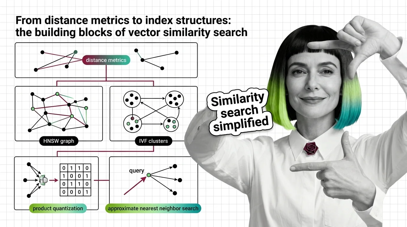
Table of Contents
ELI5
Vector similarity search finds the closest matches in high-dimensional space using distance metrics to measure closeness and index structures to avoid checking every single vector.
In two dimensions, finding the nearest point is trivial—you could eyeball it on graph paper. Add a third dimension and the problem barely changes. But push past a few hundred dimensions, and something curious happens: distances between points converge toward the same value, and brute-force comparison collapses under its own arithmetic. Most people assume the hard part of Similarity Search Algorithms is the math. It isn’t. The hard part is that the geometry of high-dimensional space actively works against the most intuitive approaches to finding neighbors.
The Arithmetic of Closeness
Before any index structure matters, you need a definition of “close.” That definition is less obvious than it sounds—because in high-dimensional space, the metric you choose changes which vectors count as neighbors. Three distance functions dominate Embedding retrieval, and each encodes a different geometric assumption about similarity.
What are the main components of a similarity search system?
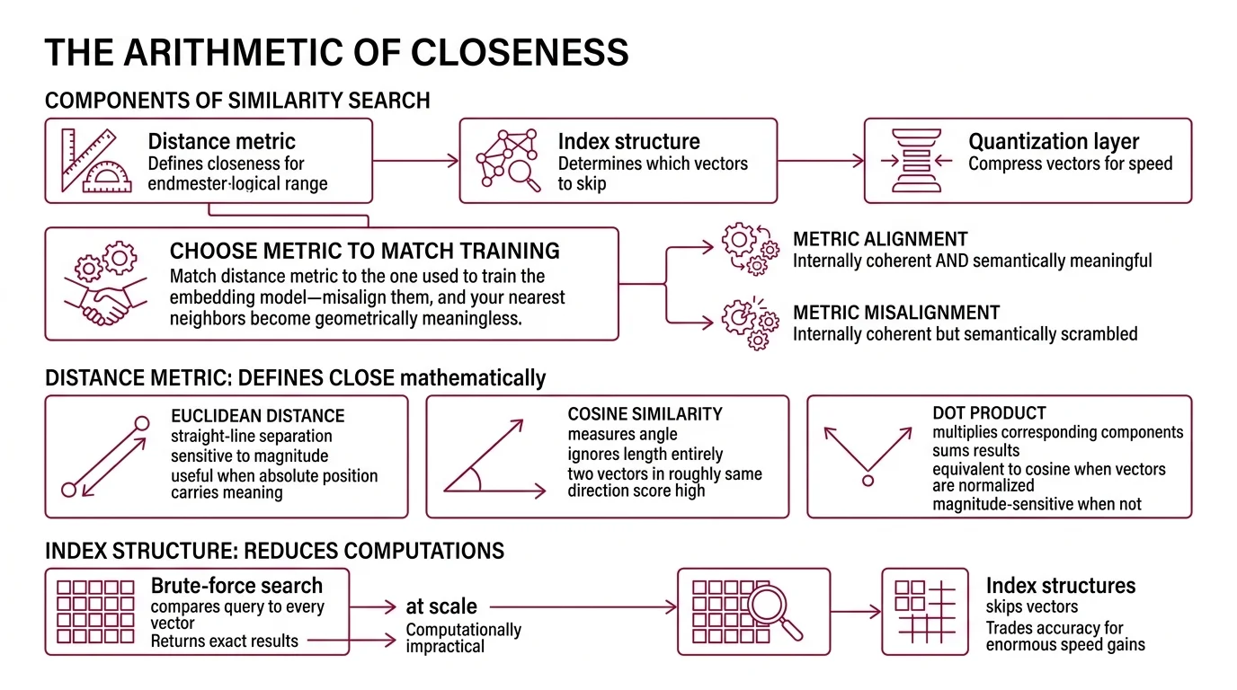
A similarity search system has three layers, each solving a different part of the problem.
The distance metric defines what “close” means mathematically. Euclidean Distance measures straight-line separation between two points—sensitive to magnitude, useful when absolute position in vector space carries meaning. Cosine similarity measures the angle between vectors, ignoring their length entirely; two vectors pointing in roughly the same direction score high regardless of how far apart they sit. The Dot Product multiplies corresponding components and sums the results—equivalent to cosine similarity when vectors are normalized, but magnitude-sensitive when they are not.
The choice is not cosmetic. Match the distance metric to the one used to train the embedding model (Weaviate Docs)—misalign them, and your nearest neighbors become geometrically meaningless. A retrieval system that returns cosine-ranked results for an embedding trained with Euclidean loss will produce orderings that are internally coherent but semantically scrambled.
The index structure determines how the system avoids computing distance against every vector in the collection. Brute-force search—comparing a query to every stored vector—returns exact results but becomes computationally impractical at scale. Index structures trade small amounts of accuracy for enormous gains in speed by deciding which vectors to skip.
The quantization layer compresses vectors to reduce memory footprint and accelerate distance computation. This is where engineering meets information theory: how much precision can you discard before the search results degrade beyond usefulness?
These three layers are not independent. The metric constrains which index structures work effectively; the index structure constrains which quantization schemes are compatible. The layers form a dependency chain, not a menu.
What math and data structure concepts do you need before learning similarity search algorithms?
The prerequisites cluster around three areas.
Linear algebra provides the foundation: vector operations, dot products, norms, and the geometric intuition that high-dimensional vectors are points in space where angles and distances carry semantic meaning. Without this, the distance metrics are formulas rather than ideas.
Probability and hashing matter for understanding locality-sensitive hashing—specifically, how hash functions can be designed so that similar inputs collide more often than dissimilar ones. The insight is statistical: similarity becomes a probability of collision rather than a deterministic distance.
Graph theory underlies the dominant modern approach. HNSW builds a navigable graph where nodes are vectors and edges connect approximate neighbors. Understanding greedy search on graphs—how a local decision at each node can lead to a globally good result—is the key intuition that makes the algorithm legible.
If you are comfortable with matrix multiplication, cosine similarity, and breadth-first search, you have enough to read the primary papers. The rest is engineering trade-offs—which is where the interesting decisions live.
Three Architectures for an Impossible Search
Once you have defined distance, you face the real engineering constraint: you cannot compute it against every vector in a billion-row collection and still respond in milliseconds. The question becomes how to structure the search so that most vectors are never examined at all. Three families of index structures have emerged, each encoding a fundamentally different strategy for approximation.
What is the difference between HNSW, IVF, and LSH index structures for similarity search?
HNSW (Hierarchical Navigable Small World graphs) builds a multi-layer proximity graph where each layer is a progressively sparser version of the one below it. A search starts at the top layer—few nodes, long-range connections—and descends through layers of increasing density, refining the candidate set at each level. The result is logarithmic search scaling (Malkov & Yashunin, IEEE TPAMI 2018), though the original paper describes this as empirically demonstrated scaling behavior rather than a formally proven bound.
The critical parameter is M, the number of connections per node. Practitioner guidance places it between 16 and 64 (FAISS Docs); higher M means better recall at the cost of more memory and slower index construction. Think of HNSW as a skip list generalized to arbitrary metric spaces—the graph itself encodes the search strategy.
HNSW dominates production vector databases. Pinecone, Weaviate, Qdrant, and Milvus all offer it as a primary index type. The reason is empirical: it consistently delivers the strongest recall-speed trade-off across diverse workloads.
IVF (Inverted File Index) takes a partition-based approach. K-means clustering divides the vector space into Voronoi cells—geometric regions where every point is closer to one centroid than to any other. At query time, the system identifies the nearest cells and searches only within those partitions. The nprobe parameter controls how many cells to examine: more probes mean higher recall, fewer probes mean faster search.
IVF’s strength is simplicity and predictable resource consumption. Its weakness is that cluster boundaries are hard boundaries—a vector sitting near the edge of one cell may be closer to a query vector in an adjacent cell than to anything in its own partition. The geometry is clean, but the partitioning is lossy at every border.
LSH (Locality-Sensitive Hashing) approaches the problem through hash functions designed so that similar vectors hash to the same bucket with higher probability than dissimilar ones (Indyk & Motwani, STOC 1998). The search examines only vectors sharing a hash bucket with the query.
LSH has strong theoretical guarantees on approximation quality. In practice, however, it typically achieves lower recall than HNSW or IVF-PQ at comparable query speeds—a trade-off that has shifted adoption decisively toward graph-based methods.
Not obsolete. Theoretically elegant—and increasingly niche.
Compression as a Search Strategy
Index structures decide which vectors to evaluate. Quantization decides how much information each vector is allowed to carry—and whether that reduction makes search impossible or merely approximate. The distinction matters more than most engineers expect.
How does product quantization compress vectors for faster approximate nearest neighbor search?
Product quantization decomposes a high-dimensional vector into smaller subvectors and quantizes each one independently (Jegou et al., IEEE TPAMI 2011). Instead of storing an embedding as a sequence of floating-point numbers, PQ splits the vector into small groups of dimensions, trains a codebook for each group using k-means, and replaces each group with a compact index pointing to the nearest codebook entry.
The compression is dramatic. Each floating-point subvector collapses to a single-byte code, yielding an order-of-magnitude reduction in memory. Distance computation becomes a series of table lookups instead of floating-point multiplications.
Not magic. Lossy compression—with a geometric structure that preserves approximate distances.
PQ works because the Cartesian product of the subspace quantizers approximates the original space’s distance structure well enough for ranking. The errors tend to affect vectors that were already marginal candidates—the distortion concentrates where it matters least.
An emerging alternative, RaBitQ (Gao & Long, SIGMOD 2024), provides theoretical error bounds that classical PQ lacks and has been integrated into FAISS v1.13 and later versions. PQ remains the established standard, but the field is moving toward quantization methods with formal guarantees.
When the Geometry Turns Against You
The three layers interact—and their interactions produce failure modes that none of them exhibit in isolation.
If you choose a distance metric that mismatches your embedding model’s training objective, the index will efficiently return the wrong neighbors. Fast and wrong is worse than slow and right, because the results look plausible. If you increase nprobe in IVF to capture edge-of-cell vectors, you recover recall—but you burn the speed advantage that made IVF attractive in the first place. If you set HNSW’s M too low, the graph becomes disconnected at sparse layers and search quality degrades unpredictably. If you quantize too aggressively with PQ, the codebook distortion pushes true neighbors below the retrieval threshold.
Rule of thumb: start with the embedding model’s documented distance metric, choose your index structure based on collection size and memory budget, and tune quantization last.
When it breaks: approximate nearest neighbor search degrades silently. Unlike a crash or a timeout, returning the second-best neighbor instead of the best produces no error signal—just subtly worse downstream results that are nearly impossible to diagnose without ground-truth evaluation sets.
The Data Says
Vector similarity search is not one algorithm. It is three interlocking decisions—metric, index, quantization—where each choice constrains the next. The geometry of your embedding space dictates your metric; your scale and latency budget dictate your index; and your memory constraints dictate how much precision you can afford to discard. Get the order wrong, and no amount of parameter tuning will compensate.
AI-assisted content, human-reviewed. Images AI-generated. Editorial Standards · Our Editors