From Distance Metrics to Graph Traversal: Prerequisites for Understanding Vector Index Internals
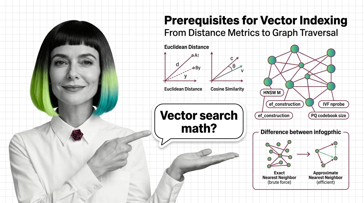
Table of Contents
ELI5
Before you can understand how vector indexes find similar items fast, you need three things: distance math that measures similarity, data structures that organize space, and the trade-off between perfect answers and fast ones.
A developer recently told me their HNSW index returned wrong results even though recall benchmarks looked reasonable. The issue had nothing to do with HNSW. It had everything to do with the distance metric they chose — or more precisely, the one they never thought about choosing. The algorithm was working perfectly. The geometry underneath it was wrong.
The Geometry That Decides Everything
Three mathematical ideas form the load-bearing structure of every Vector Indexing system. Miss any one of them, and the index will behave in ways that seem broken but are, in fact, mathematically correct — just not correct for your problem.
What math and data structure concepts do you need before learning vector indexing?
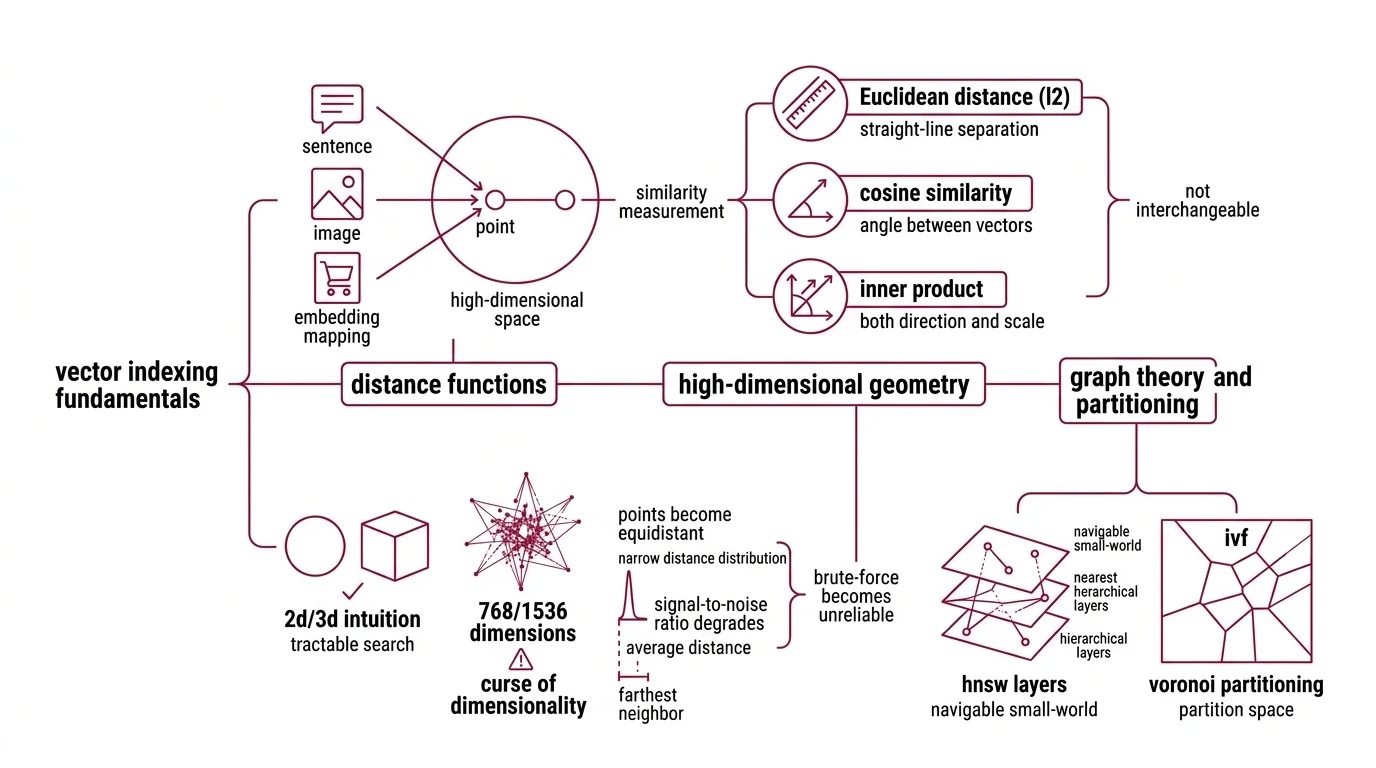
Start with distance functions. An Embedding maps your data — a sentence, an image, a product listing — into a point in high-dimensional space. Two points close together are “similar.” But “close” depends entirely on how you measure.
Euclidean distance (L2) measures straight-line separation. Cosine similarity measures the angle between vectors, ignoring magnitude. Inner product measures both direction and scale. These are not interchangeable. A pair of vectors can be close in cosine similarity and far apart in L2 if their magnitudes differ; the same data, the same vectors, different answers depending on which ruler you pick.
The second prerequisite is high-dimensional geometry, and this is where intuition betrays you. In two or three dimensions, nearest-neighbor search feels tractable — draw a circle, check what falls inside. In 768 or 1536 dimensions, something uncomfortable happens: most points become roughly equidistant from each other. The distribution of pairwise distances concentrates around a narrow band. The difference between the nearest and farthest neighbor shrinks relative to the average distance. This is the curse of dimensionality, and it explains why brute-force search doesn’t just become slow in high dimensions — it becomes unreliable, because the signal-to-noise ratio in raw distance values degrades until the gap between “relevant” and “irrelevant” nearly vanishes.
The third prerequisite is graph theory and partitioning. HNSW builds a navigable small-world graph with hierarchical layers. IVF (Inverted File Index) partitions the space into Voronoi cells using k-means clustering. Product quantization compresses vectors into compact codes using codebook lookup. Each structure encodes a different assumption about how similarity is distributed in your data — and each assumption has failure modes tied directly to the geometry above.
The Brute-Force Ceiling
There is an elegant solution to nearest-neighbor search: compare your query against every single vector in the dataset, compute the distance, return the closest ones.
It works. It is exact. And it scales as O(n * d), where n is the number of vectors and d is the dimensionality.
What is the difference between exact nearest neighbor and approximate nearest neighbor search?
Exact nearest-neighbor search guarantees you find the true closest vectors. Brute-force Similarity Search Algorithms — like flat indexes in Faiss — scan every vector, compute every distance, and return the correct answer every time (FAISS Docs). For a few thousand vectors, this is fast enough. For a few million, it becomes a bottleneck. For a billion, it is computationally intractable for real-time queries.
Approximate nearest-neighbor (ANN) search makes a different bargain. Instead of scanning everything, ANN algorithms build index structures — graphs, trees, quantized codes — that let the search skip most of the dataset. The trade-off is recall: the fraction of true nearest neighbors that actually appear in the results. A recall of 0.95 means you found 95% of the real neighbors. The remaining 5% were in regions of the space the algorithm never visited.
Not a defect. A design parameter.
The choice between exact and approximate search is the first architectural decision in any vector search system, and it depends on two things: dataset size and latency budget. If you can scan every vector within your application’s time constraint, exact search is simpler and more predictable. If you cannot — and at scale, you cannot — ANN introduces controllable imprecision in exchange for sub-linear query time. The engineering question stops being “is the answer correct?” and becomes “how much incorrectness can I tolerate, and where?”
What Each Parameter Actually Controls
Once you commit to ANN, you inherit a set of knobs. Each one governs a different axis of the quality-speed-memory triangle. Turning them without understanding the geometry underneath produces results that look like bugs but are, in fact, the parameters doing exactly what you told them to.
How do parameters like HNSW M, ef_construction, IVF nprobe, and PQ codebook size affect index behavior?
HNSW builds a layered graph where each vector connects to its nearest neighbors. Three parameters govern its behavior:
- M — the number of bidirectional links per node. Typical values range from 12 to 48; the convention default is roughly 16, though different libraries may set different defaults (hnswlib Docs). Higher M means each node is better connected, improving recall and robustness to local minima during graph traversal. The cost is direct: memory scales linearly with M, and insertion slows because each new node must evaluate more candidate connections.
- ef_construction — the size of the dynamic candidate list during index building. Values between 100 and 500 are common (hnswlib Docs). Higher ef_construction produces a better-connected graph — more accurate neighbor links — at the cost of slower build time. Once the index is built, this parameter has zero effect at query time.
- ef_search — the candidate list size during queries, which must be at least k (the number of neighbors requested). Increasing ef_search improves recall but adds latency. Unlike ef_construction, this knob is tunable after the index exists — you can adjust the recall-latency trade-off without rebuilding.
IVF partitions the vector space into clusters via k-means. At query time, the algorithm identifies the closest cluster centroids and searches only the vectors assigned to those clusters:
- nprobe — the number of clusters searched per query. It is runtime-tunable without rebuilding the index; higher nprobe improves recall at a roughly linear latency cost (Milvus Blog). The question is never “what nprobe gives the best recall” — it is “what recall is acceptable at what latency for this application.”
Product quantization (PQ) compresses each vector into a compact code by splitting it into m subvectors and replacing each subvector with the index of its nearest centroid in a learned codebook:
- m — the number of subvectors. More subvectors means finer granularity, better approximation of original distances, but larger codes and more computation during distance estimation.
- code_size — bits per subvector code. A code_size of 8 gives 256 centroids per codebook, which is the typical configuration (Pinecone Learn). Smaller code sizes compress further but distort distance estimates more severely.
The pattern across all three methods is the same: every parameter is a bet about where you want the error. M trades memory for connectivity. nprobe trades latency for coverage. code_size trades compression for fidelity. None are “set and forget” values — the optimal configuration depends on your data distribution, dimensionality, query patterns, and recall requirements.
When Foundations Fail Before Algorithms Do
The prerequisites above are not academic preamble. They predict specific failure modes.
If you choose cosine similarity for embeddings whose magnitudes carry semantic weight — magnitude-aware models where vector length encodes confidence — you discard signal before the index ever touches it. The algorithm works correctly on the distances it received. The distances were already wrong.
If your data sits in a high-dimensional space where pairwise distances concentrate (and in 768+ dimensions, they nearly always do), lowering nprobe or ef_search will not rescue recall. The index partitioned a space where “near” and “far” are barely distinguishable. You may need dimensionality reduction or a different quantization strategy before tuning the index itself.
If your vectors cluster unevenly — ten dense groups and a long tail of sparse outliers — IVF will assign most of its partitions to the dense regions and underserve the tail. HNSW handles this better because graph connectivity adapts to local density, but only if M is high enough to maintain navigable paths through sparse neighborhoods.
Rule of thumb: when recall drops below your threshold, check the geometry before blaming the algorithm. Distance metric mismatch, dimensional concentration, and cluster imbalance account for more retrieval failures than parameter misconfiguration.
When it breaks: prerequisites fail silently. A wrong distance metric does not throw an error — it returns confidently incorrect results. High-dimensional concentration does not crash the system — it erodes the gap between relevant and irrelevant results until the index cannot meaningfully distinguish them. These failures never appear in logs. They surface in downstream quality metrics, sometimes weeks after the index went live.
Compatibility notes:
- hnswlib (v0.8.0): Last release December 2023 — still functional and receiving commits, but no new PyPI release in over 15 months. Pin your version and monitor the repository.
- DiskANN (v0.49.1): The main branch is now a full Rust rewrite; C++ code has moved to the cpp_main branch. If you depend on the C++ API, verify compatibility before upgrading.
The Data Says
Vector index parameters are knobs. The prerequisites are the surface those knobs are mounted on. Distance metrics, high-dimensional geometry, and data distribution determine what “nearest” means in your system — and if that definition is wrong, no amount of parameter tuning will produce correct retrieval. Learn the geometry first. The algorithms become legible when you do.
AI-assisted content, human-reviewed. Images AI-generated. Editorial Standards · Our Editors