From Chunking to Reranking: RAG Pipeline Components and Prerequisites
ELI5
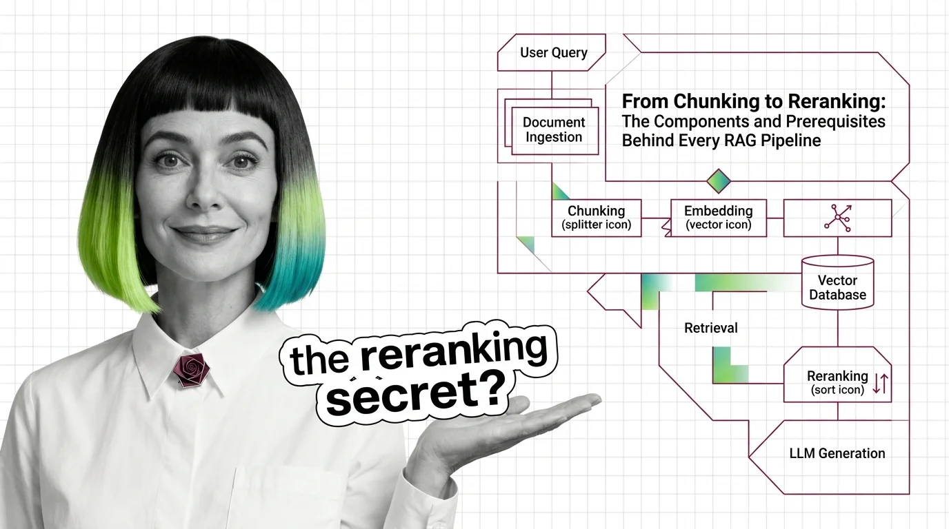
A Retrieval Augmented Generation pipeline retrieves relevant text fragments from a knowledge base, then asks a language model to answer using only those fragments. It runs as a chain of five components: chunker, embedder, vector store, retriever, and reranker.
Most engineers describe a RAG pipeline as “search plus an LLM.” Then they put one in front of users, watch it confidently cite the wrong paragraph, and realize the failure could have started in any of five places upstream of the model. The interesting part isn’t that RAG works. It’s that there are so many places where it can fail without making any noise.
This is a tour of those five places — what they do, and where each one quietly breaks.
A RAG Pipeline Is Not “Search Plus an LLM”
The original retrieval-augmented generation paper framed RAG as a way to combine parametric memory (the model’s weights) with non-parametric memory (an external corpus you can edit without retraining), per Lewis et al. (2020). That second half of the sentence is where the engineering complexity hides. A modern RAG stack is not a single retrieval call. It is a chain of transformations, and each transformation has its own characteristic failure mode.
What are the main components of a RAG pipeline?
Five components, in order of the data flow:
- Chunker — segments source documents into retrievable units. Choices about size, overlap, and boundary rules determine what the rest of the pipeline can ever see.
- Embedder — converts chunks (and queries) into numeric vectors, making text searchable by geometric similarity rather than lexical match. Embedding models are the default here.
- Vector store — indexes those vectors so that nearest-neighbor lookup runs in sub-linear time. A Vector Database like Pinecone or Qdrant handles this layer.
- Retriever — runs the query against the index and returns candidate chunks. The strongest retrievers run in Hybrid Search mode, fusing dense vector similarity with lexical signals.
- Reranker — re-scores those candidates using a heavier cross-encoder model that reads the query and chunk together, instead of comparing them as detached vectors.
Then the language model takes the top reranked chunks as context and writes the answer. Five transformations, each with a different cost profile and a different way to break.
The five-step picture fits on a slide. The reason teams still get it wrong is that the failure modes do not respect the boundaries between steps.
The Geometry of Chunking and Embedding
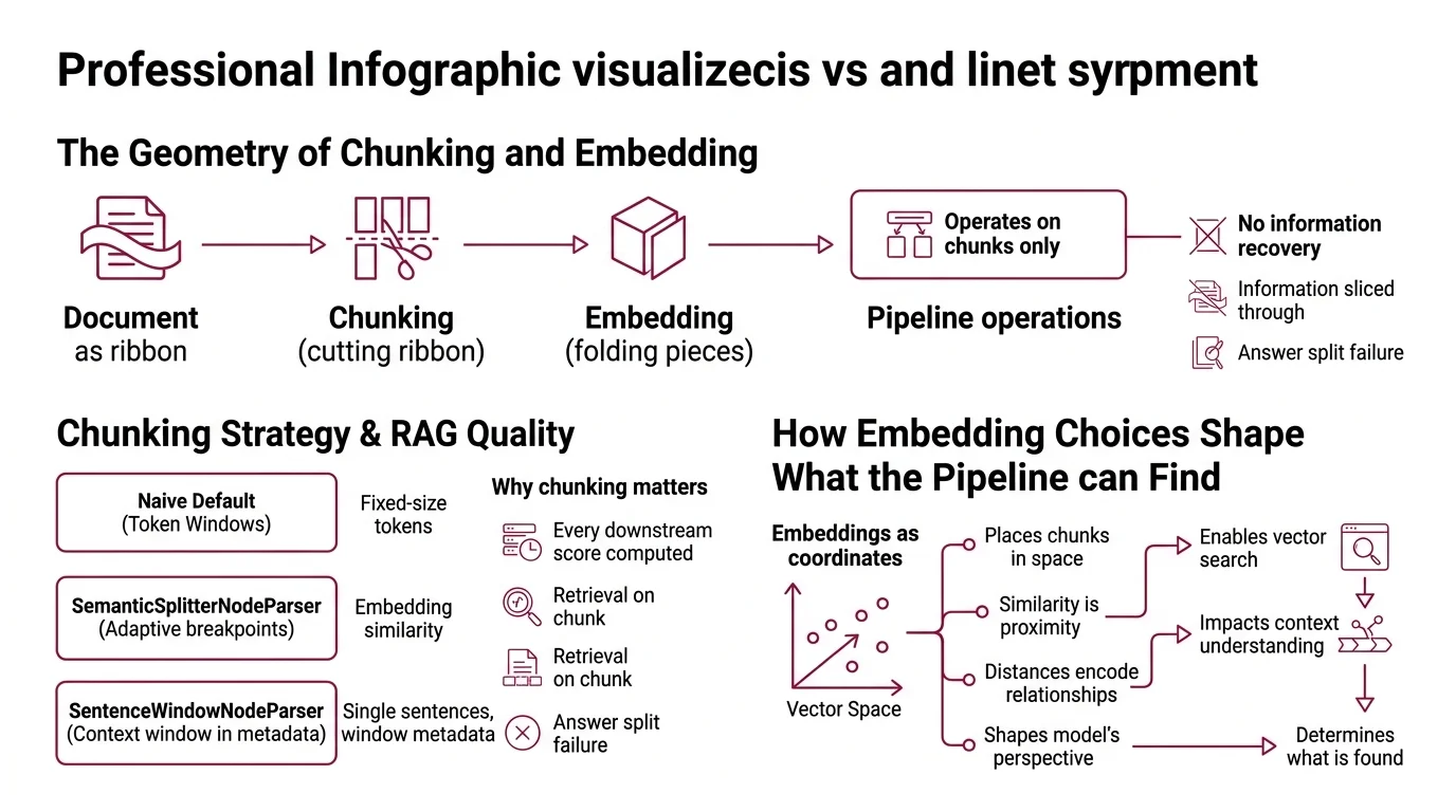
Picture every document as a long ribbon of text. Chunking is where you cut the ribbon. Embedding is where you fold each piece into a position in a high-dimensional space. Once those two steps are done, the rest of the pipeline can only operate on the pieces you produced. There is no recovering information you sliced through.
What is a chunking strategy and why is it critical to RAG quality?
A chunking strategy is the rule for how source text gets segmented before embedding. The naive default — fixed-size token windows with a small overlap — is the
LlamaIndex SentenceSplitter standard, where the default chunk size is 1024 tokens with an overlap of 20 (LlamaIndex Docs). It is fast and usually adequate for prose. It is also why a lot of pipelines fail on tables, code, and any document where a logical unit is longer than one window or sits across a window boundary.
Two more interesting strategies live in the same library. SemanticSplitterNodeParser chooses breakpoints adaptively, using embedding similarity between adjacent sentences to decide where one idea ends and another begins (LlamaIndex Docs). SentenceWindowNodeParser goes the other direction: it splits the document into single sentences for retrieval but stores a surrounding window of sentences in metadata, so the reranker and the language model see context the retriever did not have to score (LlamaIndex Docs). The
Chunking Strategy you pick decides which of these failure surfaces you accept.
The mechanical reason chunking matters so much: every downstream score is computed on the chunk, not on the document. If the answer is split across two chunks the retriever never co-retrieves, no embedding model and no reranker on earth can put it back together.
How embedding choices shape what the pipeline can find
Embeddings are coordinates, not search results. They place each chunk somewhere in a vector space, and similarity is just distance in that space. The dimension of the space matters less than people assume. OpenAI’s text-embedding-3-small produces 1,536-dimensional vectors at $0.02 per million tokens, and text-embedding-3-large reaches up to 3,072 dimensions with Matryoshka truncation that can shrink the vector to 256 dimensions with minimal quality loss (OpenAI / DeployBase). Cohere’s embed-v4 exposes a configurable output dimension in the 1024–1536 range (Cohere Docs).
A higher-dimensional embedding does not automatically search better. It searches differently. Smaller dimensions are cheaper to store and faster to compare; Matryoshka-style truncation makes the trade explicit. The pipeline question is not “which model is best” — it is “which dimensionality fits my latency, storage, and recall budget.”
Why Hybrid Retrieval Wins, and Why It Still Needs a Reranker
Once chunks are embedded and indexed, the retriever has to find them. Pure dense retrieval handles semantic similarity well — paraphrases, related concepts, fuzzy matches — and handles exact identifiers poorly: error codes, drug names, surnames, version strings. Lexical retrieval (BM25 and friends) is the mirror image: precise on identifiers, blind to paraphrases.
Hybrid retrieval fuses both. The recommended zero-config baseline is Reciprocal Rank Fusion at k=60, which combines dense and BM25 rank lists without needing labeled training data; the practical advice is to use RRF as a default, then switch to weighted convex combination once you have around fifty labeled query pairs to tune the weights against (Superlinked VectorHub).
Hybrid retrieval lifts the recall ceiling. The reranker is what turns recall into precision. A cross-encoder reranker reads the query and a candidate chunk together, in the same forward pass, and returns a fresh relevance score. This is the most expensive single component per query, and it produces the largest single precision gain in a pipeline that already has hybrid retrieval (Superlinked VectorHub).
Cohere Rerank’s current model — rerank-v3.5, served at the /v2/rerank endpoint — supports a 4096-token context across 100+ languages (Cohere Docs).
The trap is treating the reranker as a fix for a weak retriever. It cannot recover what the retriever never returned. Recall has to come first.
What You Need to Know Before You Build One
The honest list of prerequisites is shorter than most introductory blog posts pretend — and the parts people skip hurt later.
What concepts do you need to understand before learning RAG?
Four ideas, in roughly increasing order of how often they bite:
- Tokenization. Chunks are measured in tokens, not words or characters. A 1024-token chunk is roughly 700–800 English words, depending on the tokenizer. Code, math, and non-English text shift that conversion.
- Embeddings as geometry. A vector is a coordinate in a space where similar text lives close together. You do not need to understand how the embedding model was trained — but “similar” is defined by the model, and that model has its own biases about what similarity means.
- Vector similarity metrics. Cosine similarity, dot product, and Euclidean distance are not interchangeable. Most production embedders are normalized so cosine and dot product behave equivalently, but the choice still affects your index configuration.
- Approximate nearest-neighbor search. Indexes like HNSW and IVF trade a small amount of recall for a large speed-up. You do not need to implement them — you do need to know that “approximate” means your top-k is not always the true top-k, and the gap depends on the index parameters.
You do not need a deep understanding of transformer internals, attention heads, or training-time optimization. RAG is a retrieval-and-conditioning problem; the math you actually use is closer to information retrieval than to deep learning.
How much do you need to know about embeddings and vector databases before building RAG?
Less than vendor documentation suggests, and more than the typical “ten lines of LangChain” tutorial demonstrates.
For embeddings, the working knowledge is: pick a model your latency and budget tolerate, understand its dimensionality, and verify it handles the languages and domain in your corpus. You do not need to fine-tune one to start.
For vector databases, the working knowledge is shaped by an economic model that varies sharply by vendor. Pinecone’s Starter tier is free with 2 GB of storage and capped read/write units; Standard begins at $50/month with $0.33 per GB-month plus metered traffic; Enterprise begins at $500/month with private networking and HIPAA support (Pinecone’s pricing page). As of 2026, serverless is the default index type, and pod-based indexes are legacy (Pinecone Docs). Public list pricing is the floor — enterprise customers commonly negotiate prepaid credits, so treat the public number as an anchor rather than a total cost.
You do not need to know how the index is implemented. You do need to know which throughput mode you are paying for, because that decides how aggressively you can re-embed and re-index when you change your chunking strategy — and you will change it.
What This Predicts About Your First Failure
If the chunker is configured wrong, the retriever cannot fix it.
If the retriever is dense-only, exact identifiers will quietly fail to match.
If the reranker is missing, your top-k will be plausible but unfocused.
Three places to look when answer quality drops, and they tend to fail in that order.
Rule of thumb: Tune chunking before tuning anything else. The cheapest component to change has the largest effect on what every later component can do.
When it breaks: A reranker can sharpen what the retriever found, but it cannot recover documents the retriever missed — recall is set by chunking and embedding choices upstream, and no cross-encoder scoring further down the chain can compensate.
Compatibility notes:
- Pinecone pod-based indexes: Legacy as of 2026; serverless is the default for new indexes. Migration is supported only for pod indexes under 25M records and 20K namespaces (Pinecone Docs).
- Cohere Rerank-v2.0 family: Deprecated 2 December 2024 in favor of
rerank-v3.5; verify any v2 model name against Cohere’s deprecations page before using it (Cohere Docs).- LlamaIndex Python 3.9 support: Deprecated across multiple packages in March 2026 — target Python 3.10+ for new code (LlamaIndex Docs).
The Data Says
A RAG pipeline is a chain of transformations, and each transformation has its own failure mode. The components people most often get wrong are the cheapest to fix: chunk size, fusion method, and whether or not a reranker exists. The components people obsess over — embedder choice, vector database brand — matter much less than the cheap ones, as long as the pipeline above them is doing its job.
AI-assisted content, human-reviewed. Images AI-generated. Editorial Standards · Our Editors