From Binary to Multi-Class: Deriving Precision, Recall, and F1 from a Confusion Matrix

A model scores 95% accuracy on a medical screening dataset. The team celebrates. Then someone builds a confusion matrix and discovers the model predicted “healthy” for every single patient — including the 5% who actually had the disease. The accuracy was real. The model was useless. That gap between a headline number and diagnostic reality is precisely what the confusion matrix exists to close.

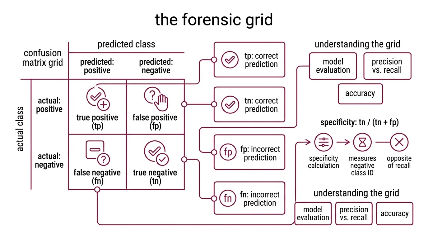
The Forensic Grid: What Each Cell Records

Every Binary Classification model produces four possible outcomes per prediction, and the Confusion Matrix arranges them into a 2×2 grid that works like a forensic report. Rows represent what actually happened; columns represent what the model claimed happened. The tension between those two axes — ground truth versus prediction — is where every interesting metric lives.

What should you understand before learning confusion matrices

The vocabulary is small but deceptively precise, and conflating any two terms will cascade errors through every metric you compute downstream.

True Positives (TP): the model predicted positive and was correct. True Negatives (TN): the model predicted negative and was correct. These occupy the diagonal — the cases where prediction aligned with reality.

False Positives (FP): the model predicted positive but was wrong. The false alarm; the spam filter that blocks a legitimate email; the fraud detector that freezes a valid transaction. False Negatives (FN): the model predicted negative but was wrong. The missed detection — the screening test that sends a sick patient home with a clean bill of health.

In scikit-learn’s convention, the matrix element C[i,j] represents the count of observations with true label i that were predicted as label j (scikit-learn Docs). For binary problems, unpacking is mechanical: tn, fp, fn, tp = confusion_matrix(y_true, y_pred).ravel(). You can also normalize the matrix — by row ('true'), by column ('pred'), or by total population ('all') — to convert raw counts into proportions, which is especially useful when class sizes differ by orders of magnitude.

Two concepts round out the foundation. Specificity — TN / (TN + FP) — measures how well the model identifies the negative class; it is the mirror of recall, focused on the opposite side of the grid. And the entire framework of Model Evaluation assumes the test set is representative of data the model will encounter in practice. When Benchmark Contamination leaks training examples into the evaluation split, every cell in the matrix inflates uniformly — the grid looks cleaner than it should, and no single metric will flag the problem because the corruption is structural, not localized.

Without clean data separation, the matrix reflects memory, not generalization.

Three Metrics, One Fundamental Tension

The grid is a ledger. Precision, recall, and F1 are the questions you pose to that ledger — and each question deliberately ignores one quadrant of the table. Understanding the arithmetic matters less than understanding what each formula leaves out.

How to calculate precision recall and F1 score from a confusion matrix

Precision = TP / (TP + FP). Of everything the model flagged as positive, how many actually were? Precision punishes false alarms. A spam filter with high precision rarely sends real email to junk — but it might let spam slip through untouched, because false negatives are invisible to this formula.

Recall = TP / (TP + FN). Of all the actual positives in the dataset, how many did the model find? Recall punishes missed detections. A cancer screening model with high recall flags most tumors — but it might also refer many healthy patients for unnecessary biopsies, because false positives sit outside this formula’s field of view.

The tension between them is mechanical, not philosophical. Lowering the classification threshold captures more true positives (recall climbs) but admits more false alarms (precision drops). Raising the threshold does the reverse. No single threshold maximizes both simultaneously — unless the model achieves perfect class separation, which in practice it almost never does. Plotting precision against recall across all thresholds produces the PR curve, and the area under that curve gives you a threshold-independent summary of model performance on the positive class. But even the PR curve is a projection; it collapses the four-cell grid into a two-dimensional trade-off and discards true negatives entirely.

Precision, Recall, and F1 Score resolves this tension through the harmonic mean: F1 = 2 × TP / (2 × TP + FP + FN). Why harmonic rather than arithmetic? Because the harmonic mean punishes asymmetry. If precision is 0.95 and recall is 0.10, the arithmetic mean is a generous 0.525. The harmonic mean returns 0.18 — a verdict that reflects how catastrophically the model fails on one dimension.

Not a design choice. A mathematical property of the harmonic mean.

The F1 score weights precision and recall equally, which is appropriate when false positives and false negatives carry similar costs. When they do not — and in most applied contexts, they do not — the F-beta score generalizes the formula: F_β = (1 + β²) × (precision × recall) / (β² × precision + recall). Setting β = 2 weights recall twice as heavily as precision; β = 0.5 does the reverse (scikit-learn Docs). A medical screening system that cannot afford missed detections should optimize for F2. A content moderation system that cannot afford wrongful removals should lean toward F0.5.

The formula is a knob. The confusion matrix is the instrument panel that tells you which direction to turn it.

Beyond Two Labels: N Classes, N² Cells

Binary classification is a special case — a useful pedagogical starting point, but not what most classification problems look like once they reach real data. When a model sorts inputs into three, ten, or a hundred categories, the 2×2 grid expands into an N×N matrix, and the off-diagonal cells no longer sort neatly into “false positive” and “false negative.”

How does a confusion matrix work for multi-class classification

In an N-class confusion matrix, each row still represents the true class and each column the predicted class. The diagonal counts correct classifications. Everything off the diagonal is a specific misclassification — and now the direction of the error carries diagnostic information. A handwriting model that confuses 3 with 8 is responding to geometric similarity; one that confuses 3 with 7 has a different failure mode entirely. The matrix records both the frequency and the trajectory of every mistake.

To compute precision or recall for a single class k, treat the problem as one-versus-rest: class k against everything else. Precision for class k uses column k (all predictions of k); recall uses row k (all true instances of k). But how do you collapse N separate per-class metrics into a single summary number?

Three averaging strategies exist, and each answers a fundamentally different question (scikit-learn Docs):

Micro averaging pools all true positives, false positives, and false negatives globally before computing one metric. For single-label problems, micro-F1 collapses to overall accuracy. It gives the population-level picture but is dominated by frequent classes — rare classes barely move the needle.

Macro averaging computes the metric independently per class, then takes the unweighted mean. Every class counts equally regardless of size. This is the strategy that surfaces failures on rare categories — the categories where failures tend to carry the most consequence and the least visibility.

Weighted averaging computes per-class metrics and averages them proportional to support — the number of true instances in each class. It accounts for imbalance without reducing to a single accuracy figure; a middle ground between micro’s population sensitivity and macro’s egalitarianism.

The choice is not a statistical preference. It is a declaration about whose errors you consider tolerable.

What the Diagonal Predicts and What the Margins Conceal

Turn the mechanism into predictions you can verify against your own models.

If you increase class imbalance — say the positive class drops from 30% to 3% of the dataset — precision on the minority class will deteriorate faster than recall, because the denominator TP + FP absorbs a growing share of false alarms from the majority class. Overall accuracy may barely shift. The confusion matrix will expose the entire asymmetry; accuracy will present a flattering summary.

If two classes share visual or semantic similarity, the off-diagonal cells between exactly those two classes will show elevated counts — a pattern invisible to any aggregate metric. This is diagnostic data: it points you toward where to focus annotation effort, where to engineer features, and which class boundary the model finds genuinely ambiguous rather than merely noisy.

If you switch from micro to macro averaging and the score drops sharply, the model is performing well on common classes and failing on rare ones. Macro-F1 is the metric that refuses to let majority outvote minority.

Rule of thumb: when overall accuracy looks strong but macro-F1 drops sharply below it, the confusion matrix almost certainly contains at least one minority class with near-zero recall. The headline number is real. The model’s coverage is not.

When it breaks: The confusion matrix assumes test labels are correct. In domains with high annotator disagreement — radiology reads, sentiment classification, legal document tagging — the matrix reflects labeling inconsistency as if it were model error. A cell showing persistent confusion between two categories might reveal a genuine model limitation, or it might reveal that human experts cannot reliably distinguish those categories either. Without measuring inter-annotator agreement first, the confusion matrix cannot separate model confusion from label ambiguity.

Compatibility note:

• scikit-learn plot_confusion_matrix: Deprecated since version 1.0. Use ConfusionMatrixDisplay.from_predictions() or ConfusionMatrixDisplay.from_estimator() instead.

The Data Says

The confusion matrix is not a metric. It is the raw evidence from which every classification metric is derived. Precision, recall, F1, specificity, balanced accuracy — all of them are different projections of the same N×N grid. And the averaging strategy you select for multi-class problems is not a statistical convenience; it is a decision about whose errors matter enough to measure.