From Autoencoders to KL Divergence: Prerequisites and Hard Limits of Variational Autoencoders
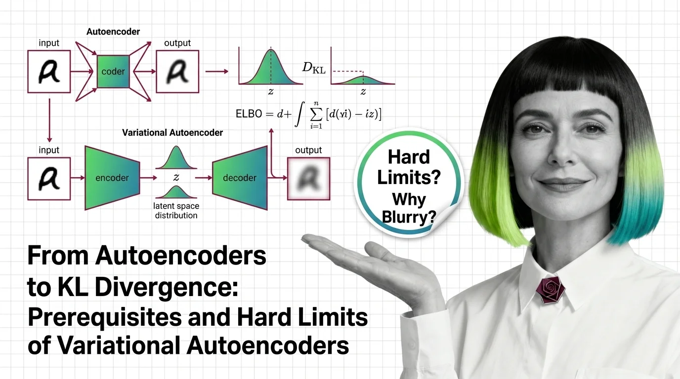
Table of Contents
ELI5
A ** Variational Autoencoder** adds controlled randomness to compression. Instead of mapping input to one fixed point, it maps to a probability region — letting the model generate new data, not just reconstruct what it has already seen.
Most tutorials introduce the variational autoencoder as a generative model. Then, in the next breath, they show blurry face reconstructions and move on to GANs. The interesting question is not why VAEs blur — it is why the same architecture became the critical compression stage inside every major diffusion system running today. That answer sits in the math most people skip.
The Geometry of Compression vs. Generation
An autoencoder is a straightforward bargain: compress an input down to fewer dimensions, then reconstruct it. An encoder network squeezes; a decoder network expands. If the reconstruction is close enough to the original, the bottleneck — the latent representation — captures something meaningful about the data’s structure.
Think of it as a postal code. The full address has street name, building number, floor, apartment. The postal code compresses that into a handful of digits. Enough to route mail to the right district; not enough to reconstruct the full address from scratch.
Difference between autoencoder and variational autoencoder
A standard autoencoder learns a deterministic mapping: input goes in, one specific latent vector comes out. Train it on faces and each face lands at exactly one point in latent space. The trouble is that the space between those points is meaningless. Pick a random coordinate between two known faces and the decoder produces noise — not a face, not anything coherent. The latent space has structure only where the training data sits.
A core Neural Network Basics for LLMs principle applies here: the network’s architecture determines what it can represent, but the training objective determines what it actually learns. Standard autoencoders optimize for reconstruction alone. VAEs add a second constraint.
The variational autoencoder, introduced by Kingma & Welling in 2013, replaces the single-point mapping with a distribution. Instead of encoding an input as a vector z, the encoder outputs two vectors: a mean (μ) and a variance (σ²). The model then samples from that distribution to produce the latent code.
The space between training points becomes navigable. You can interpolate, sample, generate — because the training process forces overlapping distributions across the latent space. The decoder does not memorize specific inputs; it learns a continuous map from probability to data.
Not compression. Structured compression with a generative license.
Three Equations That Make Randomness Trainable
There is a reason most VAE tutorials lose readers at the math section: three separate concepts converge in a single loss function, and each one solves a different problem. Separating them is more useful than memorizing the combined formula.
What math concepts do you need to understand variational autoencoders
The prerequisite list: probability distributions, Bayes’ theorem, KL Divergence, the Evidence Lower Bound, and the Reparameterization Trick.
KL divergence measures how much one probability distribution differs from another. In VAE training, it quantifies the gap between the encoder’s approximate posterior q(z|x) and a chosen prior p(z) — typically a standard Gaussian. Minimizing this term prevents the encoder from clustering all latent codes in one narrow region of space; it forces a smooth, organized latent geometry.
The evidence lower bound is the actual training objective. Maximizing ELBO pushes the model toward two goals simultaneously: reconstruct the input faithfully (the reconstruction term) and keep the approximate posterior close to the prior (the KL term). These goals pull in opposite directions — perfect reconstruction demands sharp, narrow distributions concentrated around each input; the KL penalty demands broad, overlapping ones that blend into the prior. The balance between them defines every trade-off a VAE encounters.
The reparameterization trick solves an engineering problem that the math alone cannot. You cannot backpropagate gradients through a random sampling operation — the sampler has no parameters to update. Kingma & Welling’s solution: rewrite z = μ + σ · ε, where ε is drawn from a fixed standard normal. The randomness shifts to an input (ε) that does not participate in gradient computation; the learnable parameters (μ and σ) pass gradients cleanly (Kingma & Welling).
The reparameterization trick is the reason VAEs exist as a practical method rather than a theoretical curiosity.
The Pixel Tax: Where the Blur Comes From
Ask a working ML engineer what is wrong with VAEs and you will hear one word: blurry. It is the architecture’s most famous failure — and it follows directly from the reconstruction loss, not from some avoidable design choice.
Why do VAEs produce blurry images compared to GANs and diffusion models
L1 and L2 reconstruction losses penalize pixel-level deviation between input and output. When the model is uncertain about a pixel’s value — and with probabilistic sampling, it is always somewhat uncertain — the optimal strategy under these losses is to predict the average. Averaging smooths out fine texture, high-frequency edges, the exact grain that makes an image look crisp (Saxena et al.).
The loss function punishes risk, and detail is risk.
A Convolutional Neural Network in the decoder can recover some spatial structure, but it cannot invent details the loss function penalizes it for guessing wrong. Posterior collapse compounds the problem: when the KL term dominates training, the encoder’s distributions converge toward the prior, and the latent codes carry almost no information about the input. The decoder reverts to generating the dataset’s mean image — the ultimate blur.
GANs bypass this entirely. An adversarial loss replaces pixel-by-pixel comparison with a learned discriminator that evaluates whether an output looks real. The generator can hallucinate plausible details — sharpness emerges because the discriminator penalizes blurriness as fake. The trade-off: mode collapse, where the generator finds a few safe outputs and ignores the rest of the distribution; and training instability, where the generator-discriminator equilibrium oscillates rather than converging (Saxena et al.).
Diffusion models take a different path. Progressive denoising through a U-Net recovers detail at each step — the model predicts and removes noise rather than reconstructing all pixels in one pass. No averaging over uncertainty; instead, iterative refinement that preserves high-frequency structure. Image quality surpasses both VAEs and GANs, but inference is slow — each image requires tens or hundreds of forward passes (Saxena et al.).
A Recurrent Neural Network approach to sequential generation shares the iterative logic of diffusion — building output step by step — but diffusion models operate in continuous pixel space, refining the entire image at once rather than producing a left-to-right sequence, which changes the mathematics fundamentally.

What the Latent Space Actually Predicts
If you change the reconstruction loss from L2 to a perceptual loss, expect sharper outputs — because you are moving away from pixel-level averaging toward feature-level similarity. Increase the weight on the KL term, and the latent space becomes more regularized but reconstruction quality drops. Train with very high-dimensional latent spaces, and the KL constraint weakens until the model drifts toward a standard autoencoder without generative capability.
These are not design suggestions. They are predictions that follow from the equations.
The most consequential prediction turned out to be architectural. VAEs compress images to a lower-dimensional latent space — a 512×512 image might become a 64×64 latent representation. Rombach et al. recognized that the diffusion process does not need to operate in pixel space; running denoising in the VAE’s latent space cuts computation dramatically while preserving image quality (Rombach et al.). This is the engine behind Stable Diffusion, FLUX, and most production image generators as of 2026.
The VAE’s blurriness stops mattering when its role is compression, not final generation. The diffusion model handles detail; the VAE handles dimensionality.
VQ-VAE offered another escape from the blur problem: replace continuous distributions with discrete codebook vectors (van den Oord et al.). No KL divergence against a Gaussian prior; no averaging. The codebook learns a vocabulary of visual features, and the decoder reconstructs from discrete codes. Posterior collapse vanishes because the training mechanism is fundamentally different — vector quantization rather than distribution matching.
When it breaks: The ELBO’s reconstruction-KL tension means you can optimize for better reconstruction or a more organized latent space, but not both simultaneously beyond a certain frontier. Posterior collapse remains the most common training failure in practice, and diagnosing it requires monitoring both loss terms independently — the combined loss can decrease while generative quality degrades silently.
A recent line of work suggests the VAE component may become removable entirely. Shi et al. proposed SVG at ICLR 2026, replacing the trained VAE encoder with a frozen self-supervised encoder (DINOv3) and a learned decoder — eliminating the need for a trained VAE in the latent diffusion pipeline. Real-world adoption of this approach remains unknown, but the direction signals that the VAE’s role as latent compressor is not necessarily permanent.
The Data Says
The variational autoencoder is a compression architecture with a generative license, granted by three mathematical components — KL divergence, ELBO, and the reparameterization trick. Its blurriness is not a flaw in implementation but a consequence of the loss function asking the model to hedge every pixel. Understanding the prerequisites — what each equation does and what it sacrifices — is the difference between using VAEs as a black box and knowing when to replace them.
AI-assisted content, human-reviewed. Images AI-generated. Editorial Standards · Our Editors