Diminishing Returns, Data Exhaustion, and the Hard Technical Limits of Neural Scaling
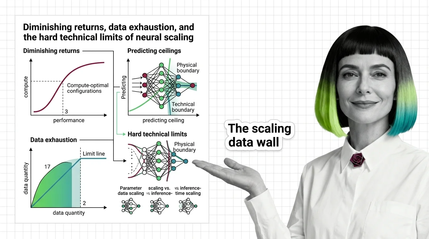
Table of Contents
ELI5
Scaling laws describe how model performance improves as you add compute, data, or parameters — but the gains shrink logarithmically. Eventually, the planet runs out of text before the math runs out of room.
In 2020, a team at OpenAI plotted loss against compute on a log-log scale and watched a straight line appear. The finding felt almost too clean: multiply compute by ten, and performance improves by a fixed fraction — not tenfold, a fraction. The line was beautiful. Its slope was the problem.
The popular narrative treats scaling as a promise: spend more, get more. Most discussions about Scaling Laws focus on whether they hold. A more uncomfortable question is what happens when they do — because a power law with an exponent below one is not a temporary inconvenience. It is a mathematical guarantee of diminishing returns, baked into the exponents themselves.
Power Laws and the Slope Nobody Advertises
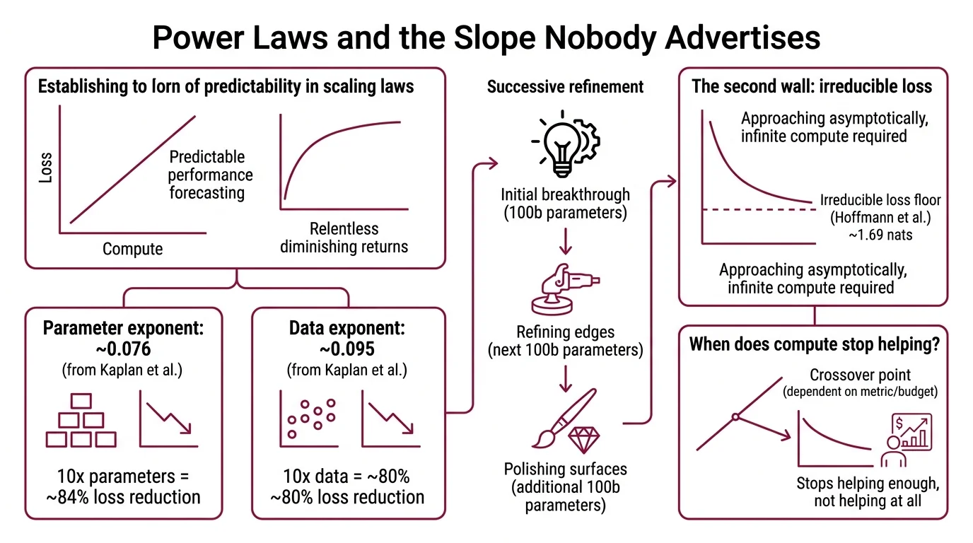
The appeal of scaling laws is their predictability. Plot training loss against compute, parameters, or data on logarithmic axes, and the relationship is approximately linear. That linearity lets you forecast performance before spending the compute. But forecasting diminishing returns is still forecasting diminishing returns.
Why do scaling laws show diminishing returns and when does adding more compute stop helping?
The original scaling analysis measured the exponents precisely: the parameter exponent sits at roughly 0.076 — meaning a tenfold increase in parameters reduces loss to about 84% of its previous value (Kaplan et al.). The data exponent is slightly steeper at 0.095; ten times more data drops loss to roughly 80% (Kaplan et al.).
These numbers sound modest because they are.
A power-law exponent below one means each successive unit of resource buys less improvement. The first hundred billion parameters transformed what language models could do. The next hundred billion refined the edges. The hundred billion after that polished surfaces most users never notice.
The mechanism isn’t mysterious — it’s geometric. On a log-log plot, constant exponents produce straight lines. On a linear plot, those same lines are curves that flatten relentlessly. The math doesn’t bend. Your expectations do.
There is a second wall: irreducible loss. The Chinchilla analysis estimated an irreducible loss floor of approximately 1.69 nats — the entropy of natural language itself (Hoffmann et al.). No amount of scaling eliminates noise intrinsic to the data distribution. You can approach that floor asymptotically, but asymptotic approach and arrival are different concepts separated by infinite compute.
When does adding more compute stop helping? Strictly speaking, it never stops helping — it stops helping enough. The crossover point depends on what you’re measuring and what you’re willing to spend, but the shape of the curve is not negotiable.
The Calculus of Compute-Optimal Training
Knowing that scaling yields diminishing returns raises a sharper question: given a fixed compute budget, how should you allocate it between model size and training data? The answer depends on which paper you trust — and how carefully you read the exponents.
How do researchers estimate compute-optimal training configurations and predict scaling ceilings?
Kaplan et al. proposed an allocation rule: scale parameters faster than data. Their formula suggested optimal model size scales as C^0.73, meaning most of a compute increase should fund bigger models. Data scaling was secondary, proportional to C^0.27.
Hoffmann et al. disagreed. Their Chinchilla Scaling analysis arrived at a fundamentally different allocation: scale model size and data equally, with both proportional to C^0.5. The validation was decisive — a 70-billion-parameter model trained on four times the data outperformed the 280-billion-parameter Gopher, achieving 67.5% on MMLU, a seven-percentage-point improvement (Hoffmann et al.).
That result reshaped how labs budget for Compute Optimal Training.
But the Chinchilla result is not beyond scrutiny. A 2024 replication attempt found that the third estimation procedure in the original paper produced inconsistent results with implausibly narrow confidence intervals, and revised exponent fits differed from the originals (Epoch AI Replication). The core insight — that Kaplan’s allocation was too parameter-heavy — has held across subsequent work. The precise exponents remain a moving target.
Predicting ceilings requires a different input entirely: data supply. Epoch AI’s central estimate puts the total stock of quality text at roughly 300 trillion tokens, though the 90% confidence interval spans from 100 trillion to one quadrillion tokens — a range so wide it borders on confession (Epoch AI). Under compute-optimal assumptions, this stock saturates at approximately 5 x 10^28 FLOP, a threshold the field may reach around 2028. Overtraining accelerates the timeline: at five times the compute-optimal data ratio, exhaustion moves to 2027; at one hundred times, it would have arrived by 2025 (Epoch AI).
The ceiling isn’t just computational. It’s ecological.
Three Budgets, Three Walls
Not all scaling is the same kind of spending. The distinction between parameter scaling, data scaling, and Inference Time Scaling determines which ceiling you hit first — and whether you can route around it.
What is the difference between parameter scaling, data scaling, and inference-time scaling?
Parameter scaling means adding more weights to the network. More parameters increase the model’s capacity to represent complex functions, but each additional parameter contributes less than the one before it — the power-law exponent guarantees this. At current frontier scale, parameter increases primarily refine performance on tasks the model already handles reasonably well. Emergent Abilities — capabilities that appear suddenly at certain parameter thresholds — remain contested; some researchers argue they are artifacts of discontinuous evaluation metrics rather than genuine phase transitions in the underlying model.
Data scaling means training on more tokens. The Chinchilla insight showed that most models before 2022 were undertrained relative to their size — they had more capacity than their data could fill. But data scaling faces a hard physical constraint: the total volume of quality human-generated text is finite. Synthetic data offers a partial workaround, though models trained on their own outputs risk distribution narrowing — each successive generation loses variance the original corpus contained.
Inference-time scaling is the newest axis, and it operates under fundamentally different economics. Instead of training a bigger model, you spend more compute at inference to let the model reason longer. The o3 system demonstrated this dramatically: the high-compute configuration used 172 times more compute than the low configuration, generating roughly 57 million tokens per question versus 330 thousand (Cameron R. Wolfe). DeepSeek-R1 showed that reinforcement learning alone — at a fraction of frontier Pre Training cost — could produce strong reasoning capability.
The inference-time approach reframes the scaling question entirely. Instead of asking “how large should the model be?”, it asks “how long should the model think?” — and the answer can vary per query, per user, per difficulty level. Inference compute is the newest frontier because it sidesteps both the parameter ceiling and the data ceiling. Whether this constitutes a genuinely different scaling regime or simply moves the cost from training to deployment remains an open empirical question.
What the Exponents Predict
If you accept the power-law framework, several engineering consequences follow — and they are less dramatic than the scaling narrative suggests.
If you increase your compute budget by an order of magnitude and allocate it optimally, the resulting loss reduction is real but incremental — a matter of single-digit or low-double-digit percentage points, depending on allocation. The gains compound across many orders of magnitude, but the lived experience at any single step is modest.
If you’re choosing between a larger model and more training data, the Chinchilla allocation — roughly equal scaling — remains the best available default, despite the replication caveats. Most frontier models since 2023 have followed some variant of this ratio.
If you need capability gains without scaling parameters or data, inference-time scaling offers an alternative path — but at the cost of per-query latency and compute expenditure. The economics shift from capital expenditure on training to operational expenditure on inference.
If you’re building on Fine Tuning or RLHF, recognize that these techniques operate within the capability envelope that pre-training established. They redistribute the model’s probability mass across outputs; they don’t expand the envelope’s radius. The most common engineering mistake is treating post-training as if it adds capabilities. It surfaces capabilities the base model already possesses — it cannot conjure abilities the pre-training distribution never contained.
Recent work adds a critical caveat: upstream loss improvements don’t reliably predict downstream benchmark gains (ACL 2025). A model with lower perplexity may not score higher on the specific task you care about. Scaling laws describe loss, not capability.
When it breaks: Scaling laws assume the data distribution is fixed and the architecture is held constant. Change the architecture — mixture-of-experts, retrieval augmentation, test-time compute — and the exponents shift. The laws describe one regime, not all possible regimes. Extrapolating a power law past its observed range is a bet, not a proof.
Rule of thumb: Tenfold more parameters reduces loss to roughly 84% of its previous value; tenfold more data to about 80%. These are the best-case conversion rates — and they are sublinear by design.
The Data Says
Scaling laws are among the most robust empirical findings in machine learning — and among the most frequently misread. They don’t promise exponential progress. They promise predictable, decelerating progress. The exponents are small, the irreducible loss floor is real, and the planet’s text supply is finite. The field has already begun routing around these limits through inference-time scaling, but that trades one ceiling for another. Understanding the shape of the curve is not pessimism — it is the prerequisite for building anything that lasts.
AI-assisted content, human-reviewed. Images AI-generated. Editorial Standards · Our Editors