Dense vs. Sparse, Cosine vs. Dot Product, and the Technical Limits of Vector Representations
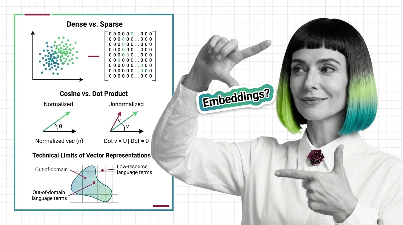
Table of Contents
ELI5
Embeddings turn words into lists of numbers. Dense ones pack meaning into every slot; sparse ones light up only specific words. The ruler you choose to measure distance between them decides which search results you trust.
Take two vectors representing the same sentence. Measure the angle between them — identical. Multiply their magnitudes — suddenly one is “closer” to a third, unrelated vector. You changed nothing about the meaning. You changed the ruler. And the ruler lied.
This is not a theoretical curiosity. It is the geometry underneath every Embedding search you have ever run, and it determines whether your retrieval pipeline returns the right document or a confident impostor.
Two Alphabets for the Same Reality
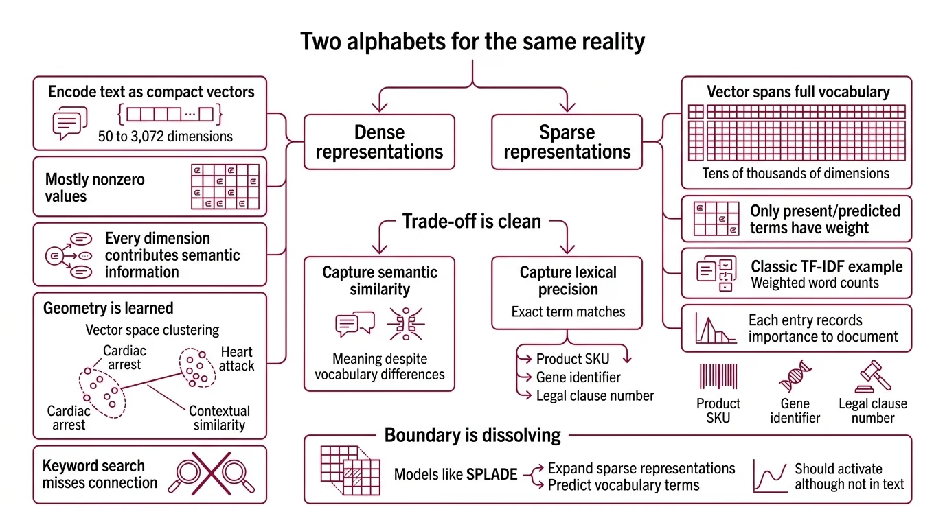
Think of two different ways to spell the same word. One alphabet uses a fixed set of characters — every position occupied, every dimension carrying a fraction of the meaning. The other uses a dictionary-sized grid where only a handful of cells light up, each one pointing directly at a specific word in the vocabulary.
That is the structural difference between dense and sparse embeddings — and the reason they fail on different inputs.
What is the difference between dense embeddings and sparse embeddings?
Dense Dense Retrieval representations encode text as compact vectors — typically 50 to 3,072 dimensions with mostly nonzero values (Zilliz Learn). Every dimension contributes a fragment of semantic information. The geometry is learned: words that appear in similar contexts cluster nearby in the vector space, even when they share no surface characters. “Cardiac arrest” and “heart attack” occupy neighboring regions; a keyword search would miss the connection entirely.
Sparse representations take the opposite approach. A sparse vector spans the full vocabulary — tens of thousands of dimensions — but only the dimensions corresponding to present or predicted terms carry nonzero weight. Classic TF-IDF is the textbook example: each nonzero entry records how important a specific word is to that document relative to the corpus.
The trade-off is clean.
Dense embeddings capture semantic similarity — meaning despite vocabulary differences. Sparse embeddings capture lexical precision — exact term matches that dense models routinely miss. A product SKU, a gene identifier, a legal clause number: these are signals that live in the sparse alphabet and barely register in the dense one.
The boundary between the two alphabets is dissolving. Models like SPLADE learn to expand sparse representations beyond the literal tokens — predicting which vocabulary terms should activate even though they don’t appear in the text. It is a sparse vector that has learned to guess the right words.
Not guessing. Learned lexical expansion.
The hybrid instinct
Production retrieval systems increasingly combine both alphabets. A dense pass captures semantic neighbors; a sparse re-ranking pass verifies lexical alignment. The reason this works is geometric: the two representations encode orthogonal signals. Fusing them covers failure modes that neither alphabet handles alone — semantic drift on one side, vocabulary mismatch on the other.
Three Rulers Measuring Different Things
You have a vector. Your Vector Database holds millions of vectors. You need the closest ones. The question nobody asks early enough: closest by what definition?
Three distance functions dominate the field. They agree less often than you would expect.
How do cosine similarity, dot product, and Euclidean distance compare for embedding-based search?
Cosine Similarity measures the angle between two vectors, ignoring their length entirely. A whisper and a shout pointing the same direction score identically — only orientation matters. It ranges from -1 (opposite) to 1 (identical direction), and it is the default choice when you care about topical similarity regardless of document length or embedding magnitude (Pinecone).
Dot product measures both direction and magnitude. When two vectors are L2-normalized — scaled to unit length — dot product and cosine similarity produce mathematically identical rankings. But without normalization, magnitude becomes a vote. A scaled-up copy of vector x can rank closer to x than x ranks to itself (Weaviate). That is not a bug in the math; it is the math working correctly on inputs you did not intend to give it.
Euclidean distance measures the straight-line gap between two points in the space. It is intuitive in two or three dimensions. In high-dimensional space, intuition breaks: a single outlier dimension with a large irrelevant value can dominate the entire distance calculation (Pinecone), drowning out hundreds of meaningful dimensions that carry the actual semantic signal.
| Metric | Measures | Ignores | Failure Mode |
|---|---|---|---|
| Cosine similarity | Direction (angle) | Magnitude | Insensitive to vector confidence |
| Dot product | Direction + magnitude | Nothing (both contribute) | Magnitude bias without normalization |
| Euclidean distance | Point-to-point gap | Directional alignment | Outlier dimension dominance |
The practical rule: match the metric to the one used during training (Weaviate). An embedding model optimized for cosine similarity during its contrastive learning phase has arranged its geometry around angular relationships. Measuring that geometry with Euclidean distance is like using a thermometer to check wind speed — the instrument is precise, but it is measuring the wrong property.
When vectors are normalized, all three metrics rank identically. Cosine equals dot product; Euclidean reduces to a monotonic function of cosine. The choice collapses into a formatting question rather than a mathematical one.
Where the Map Fails to Match the Territory
Every embedding model carries a hidden assumption: that the vector space it learned is representative of the text you will ask it to encode. When that assumption holds, the geometry is reliable. When it breaks, the failures are silent, systematic, and — here is the uncomfortable part — indistinguishable from correct results without external validation.
Why do embedding models fail on out-of-domain text, rare terms, and low-resource languages?
Three failure modes, each rooted in a different geometric deficiency.
Domain shift. An embedding model trained on web text has learned a geometry of general English. Feed it a patent filing, a radiology report, or a Kubernetes error log, and the vectors it produces occupy regions of the space that were sparsely populated during training. The distances between those vectors carry less information — the geometric neighborhood was never calibrated for that terrain. Results look plausible. They are plausible in the way a confident guess is plausible.
Rare terms. Subword tokenizers fragment unfamiliar words into arbitrary pieces, scattering them across embedding dimensions that were trained to represent more common subword units. The resulting vector is a mosaic of unrelated fragments. It points somewhere in the space, but “somewhere” is not “the right place.”
Low-resource languages. Fine-tuning data remains nonexistent for many languages; models trained predominantly on English and a few high-resource languages produce embeddings for low-resource text that cluster too tightly, collapsing distinctions that make retrieval meaningful (arxiv).
There is a deeper structural issue. In high-dimensional spaces, a phenomenon called hubness distorts the nearest-neighbor graph entirely. Certain vectors become disproportionate “hubs” — appearing as nearest neighbors far more often than statistical expectation would predict (Radovanovic et al.). These hubs degrade retrieval quality, classification accuracy, and clustering coherence simultaneously. Dimensionality Reduction can mitigate the effect, but it introduces its own information loss — a geometric tax with no free exemptions.
The Geometry Has Consequences
If you switch from cosine similarity to unnormalized dot product without re-indexing, expect longer documents and higher-magnitude vectors to dominate your results — not because they are more relevant, but because they are louder.
If you feed domain-specific text into a general-purpose embedding model, expect retrieval degradation that shows up as plausible but incorrect results. The vectors will be close in the space. They will be close for the wrong reasons.
If your corpus contains rare identifiers — part numbers, chemical formulas, API endpoint paths — a pure dense retrieval pipeline will smooth over exactly the details you need to match. A sparse pass catches what the dense pass blurs.
Rule of thumb: Normalize your vectors; measure with cosine; add a sparse lexical pass for any corpus that contains identifiers, codes, or domain-specific jargon that the embedding model did not see during training.
When it breaks: Matryoshka Embedding representations allow truncating vectors to fewer dimensions for speed — up to 14x smaller at equivalent accuracy (Kusupati et al.) — but the truncation discards information from the lower-priority dimensions. Below a task-specific threshold, the compressed embedding stops distinguishing documents that the full-dimensional version separates cleanly. The speed gain is real. So is the precision loss.
The Data Says
The choice between dense and sparse, between cosine and dot product, is not a preference. It is a geometric commitment — and the geometry has opinions about what your search results will look like. Match the metric to the model’s training objective, fuse sparse and dense signals where lexical precision matters, and assume that every embedding model carries a domain boundary it will not warn you about.
AI-assisted content, human-reviewed. Images AI-generated. Editorial Standards · Our Editors