Curse of Dimensionality, Recall vs. Speed, and the Hard Limits of Approximate Nearest Neighbor Search
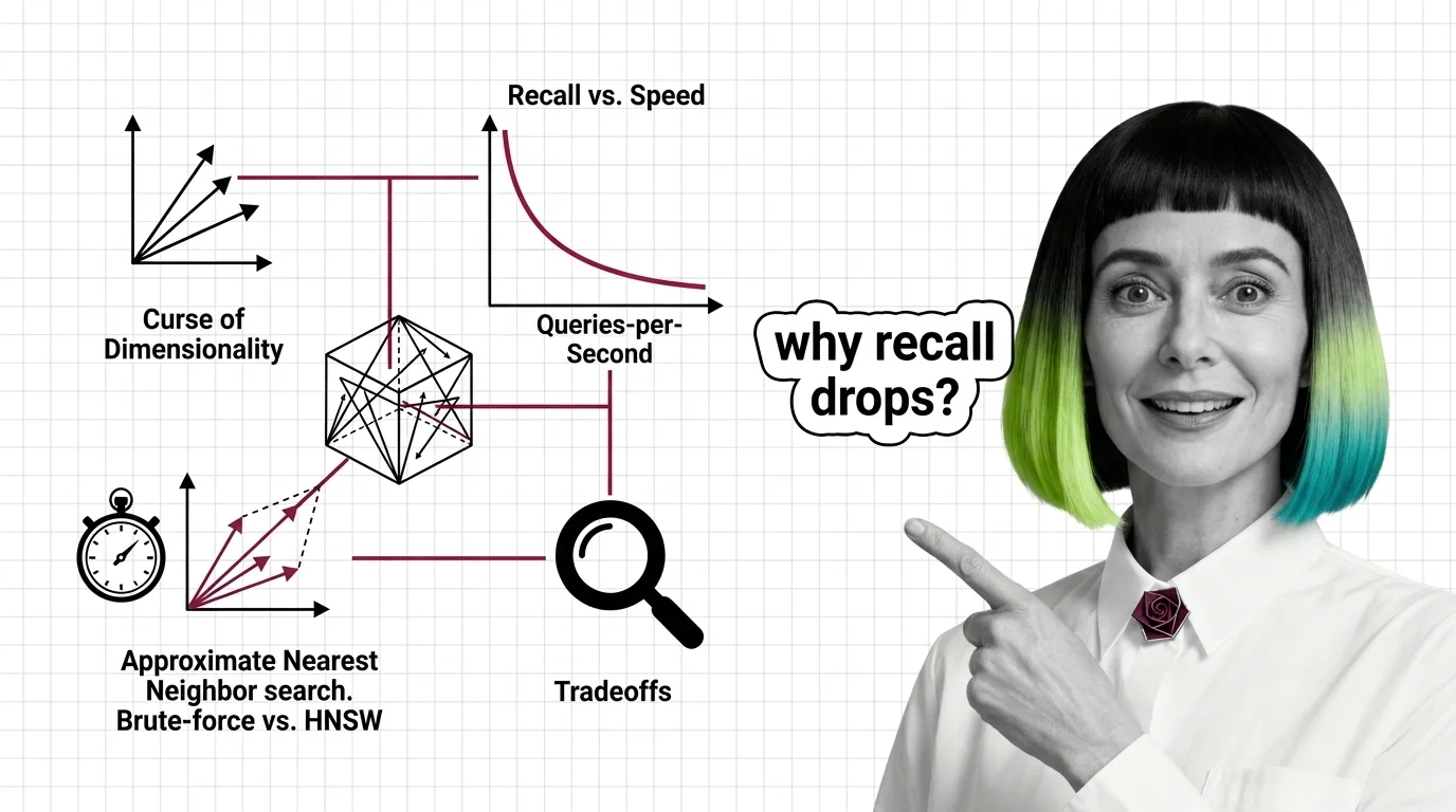
Table of Contents
ELI5
Similarity search finds the closest vectors in high-dimensional space. As dimensions grow, distances lose meaning, approximate methods trade recall for speed, and brute force sometimes wins. The math has hard limits.
Run a nearest-neighbor search in three dimensions and the closest match stands clearly apart from the crowd. Run the same search in three hundred dimensions and something unsettling happens—the nearest point and the farthest point sit almost the same distance away. Most engineers read this as a performance problem: more features, slower computation. The actual problem cuts deeper. The distances themselves stop carrying information—and the algorithms built to cope do not solve this; they negotiate with it.
The Geometry That Betrays You
Distance works differently in high-dimensional space than intuition suggests. In two or three dimensions, your distance metric is a reliable ruler—some points are genuinely close, others genuinely far, and the ratios between those distances carry meaning. Scale the dimensions past a few dozen and that ruler does not break. It goes numb.
Why does similarity search accuracy degrade in very high-dimensional spaces?
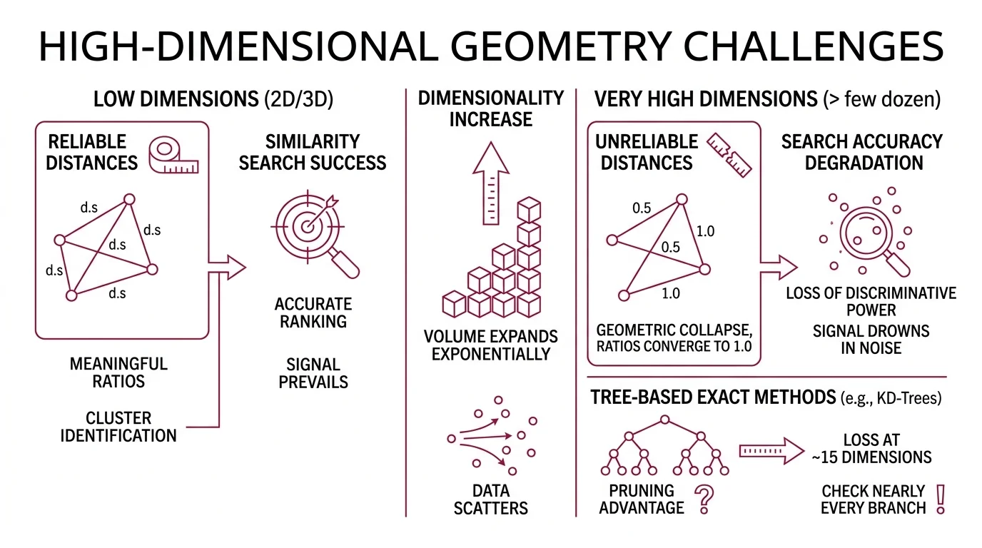
The curse of dimensionality describes a geometric collapse. As dimensions increase, the volume of the space expands exponentially while the data inside it does not. Points that appeared clustered in lower dimensions scatter into a vast, sparse void where every direction looks equally empty.
The practical consequence: Euclidean Distance and other distance metrics lose discriminative power. The ratio of the distance to the nearest neighbor versus the distance to the farthest neighbor converges toward 1.0. When your similarity metric can barely distinguish the best match from a random match, Similarity Search Algorithms face a fundamental signal-to-noise problem.
This concentration of distances is not a gradual degradation. It is a phase transition. Below a certain dimensionality—dependent on the data distribution and sample size—the nearest neighbor is meaningfully closer than the average point. Above that threshold, the signal drowns in noise. The search algorithm still returns a result; it just cannot guarantee that result is meaningfully different from a random selection.
Tree-based exact methods—KD-Trees, Ball Trees—illustrate this breakdown concretely. They partition space into regions and prune branches that cannot contain the nearest neighbor. In high dimensions, nearly every branch needs checking because all regions look equally plausible. These methods lose their pruning advantage at roughly fifteen dimensions (scikit-learn Docs); the geometric shortcuts that make tree search efficient simply vanish.
Not a software limitation. A geometric one.
But intuition misleads again here: the ambient dimensionality—the number of coordinates in your vector—is not always the dimensionality that matters. Real-world data often lies on lower-dimensional manifolds embedded within the high-dimensional space. A 768-dimensional sentence Embedding might have an intrinsic dimensionality of a few dozen. The curse bites hardest when intrinsic dimensionality is also high, not merely when the vector has many coordinates. This distinction determines whether approximate methods can exploit structure in the data—or whether the geometry is genuinely as hostile as the ambient dimensions suggest.
The Approximation Bargain
Every approximate nearest neighbor algorithm strikes the same implicit deal: give up some recall—the fraction of true nearest neighbors you actually find—in exchange for speed. The question is never whether you lose accuracy. It is how much you can afford to lose, and what the exchange rate looks like for your specific data.
What are the recall vs. queries-per-second tradeoffs in approximate nearest neighbor algorithms?
The tradeoff follows a characteristic curve, not a straight line. Recall improves quickly at first as you invest more computation, then plateaus near perfection with sharply diminishing returns. ANN-Benchmarks, the community standard for evaluating these algorithms across datasets and parameter configurations (ANN-Benchmarks), makes this shape visible: recall on one axis, queries per second on the other, and every algorithm traces its own path through that space.
HNSW—Hierarchical Navigable Small World graphs, introduced by Malkov & Yashunin in 2018—builds a layered graph where top layers provide sparse highway connections and bottom layers provide dense local links. Query time scales as O(log N), and the efSearch parameter controls where you sit on the recall-speed curve: higher efSearch means more graph nodes examined per query, higher recall, lower throughput (Malkov & Yashunin).
IVF—Inverted File Index—takes a different structural approach. It clusters the dataset using k-means, then searches only the nearest clusters at query time. The nprobe parameter determines how many clusters you examine. Searching a small fraction of clusters can maintain recall above ninety percent on well-structured datasets, though this figure is highly dataset-dependent and assumes careful nprobe tuning (Milvus Blog).
Product Quantization compresses vectors into compact codes, reducing memory by an order of magnitude at the cost of quantization error. Combined with IVF as IVF-PQ, it enables billion-scale search—Meta uses FAISS internally for searches across more than a trillion 144-dimensional vectors (Meta Engineering Blog).
Locality Sensitive Hashing takes yet another path: it hashes similar vectors into the same buckets with high probability. The seminal work by Indyk & Motwani in 1998 formalized approximate nearest neighbors with provable sublinear guarantees—at the cost of significant memory overhead for the hash table structure (Indyk & Motwani).
The shape of the curve matters more than any single benchmark result. HNSW generally achieves higher recall than IVF at comparable latency, but IVF-PQ uses a fraction of the memory. The choice is not a leaderboard competition; it is a resource allocation decision about which constraint—RAM, latency, or recall—you can least afford to violate.
When Brute Force Wins
The sophistication of approximate methods obscures a counterintuitive reality: there are common, well-defined conditions where computing every single distance—exhaustive, brute-force search—outperforms all of them. These are not exotic edge cases; they describe ordinary engineering scenarios involving small datasets, high dimensions, or infrequent queries.
When does brute-force exact similarity search outperform approximate methods like HNSW or IVF?
Brute force computes the Dot Product or Euclidean distance between the query and every vector in the dataset. No index. No approximation. No recall loss. The cost is linear in N, which sounds prohibitive—until you consider the overhead that approximate methods demand: index construction time, memory for graph or hash structures, and the parameter tuning required to find a workable operating point on the recall-speed curve.
Brute force becomes the rational choice under specific conditions: small datasets where index construction overhead exceeds the search savings it enables; dimensionality above roughly fifteen to twenty, where tree-based partitioning loses its pruning advantage; large k relative to N, where you need a substantial fraction of the dataset returned; sparse or irregular distributions that violate the clustering assumptions underlying IVF; or workloads with few total queries, where amortizing index build cost is economically irrational (scikit-learn Docs).
Exact search is the correct default until proven otherwise. FAISS makes this explicit in its architecture: the Flat index performs brute-force search and serves as the baseline against which every approximate method is measured. When your dataset fits comfortably in memory and query volume is moderate, the Flat index wins not by cleverness but by having zero overhead to amortize.
There is also a subtlety about query patterns. Approximate indices amortize their construction cost over many queries. If your application issues a burst of queries once per day against a frequently updated dataset, the index rebuild cost may dominate entirely. Brute force eliminates this maintenance burden—it requires no pre-computation, no parameter selection, no rebalancing when data changes.
The breakpoint is not a fixed number. It sits at the intersection of dataset size, dimensionality, available hardware, latency requirements, and acceptable recall loss. Engineers who skip directly to HNSW or IVF without first benchmarking brute force on their actual workload are optimizing against assumptions—not measurements.
Where the Tradeoff Curves Collapse
The implications are structural, not incremental. If you change the dimensionality of your embeddings—switching from a 384-dimensional model to a 1536-dimensional one—expect the recall-speed tradeoff to shift in ways that may require complete retuning of index parameters. The relationship is not linear.
If you increase dataset size by an order of magnitude, approximate methods pull ahead of brute force—but only if your index fits in memory. The moment you spill to disk, graph-based search collapses under I/O bottleneck and the latency advantage disappears.
If you need recall above ninety-nine percent, most approximate configurations will cost you nearly as much computation as exact search. The last few percentage points of recall are disproportionately expensive; the marginal cost of precision accelerates as you approach perfection.
If you are building a retrieval pipeline where the downstream consumer is a language model, recall takes on an asymmetric importance. A false positive—an irrelevant document in the context window—wastes tokens but causes limited harm. A false negative—a relevant document the search missed—is a silent deletion from the model’s available evidence. These failure modes are not symmetric, and your index parameters should reflect that asymmetry.
Rule of thumb: If you cannot state your minimum acceptable recall as a number, you cannot choose an index type. Start with brute force, measure the latency, and switch to an approximate method only when the measurement is unacceptable.
When it breaks: Every approximate search index silently drops true nearest neighbors. The failure is invisible—you never see the results you missed, only the ones you got. In retrieval-augmented generation pipelines, this means relevant context vanishes without error messages, and the downstream language model confabulates to fill the gap.
Security & compatibility notes:
- pgvector HNSW Buffer Overflow (CVSS 8.1): Critical vulnerability (CVE-2026-3172) in parallel HNSW index build affecting pgvector versions 0.6.0 through 0.8.1. Upgrade to a patched version before running parallel index builds.
The Data Says
Similarity search has hard mathematical limits that no algorithm eliminates—only redistributes. The curse of dimensionality degrades all distance-based methods; approximate algorithms trade recall for speed along characteristic curves that plateau near perfection; and brute force remains the rational default for small datasets, high dimensions, or when recall loss is unacceptable. The engineering question is never which algorithm is best. It is which tradeoff you can survive.
AI-assisted content, human-reviewed. Images AI-generated. Editorial Standards · Our Editors