Class Imbalance, Normalization Traps, and the Hard Limits of Confusion Matrix Analysis
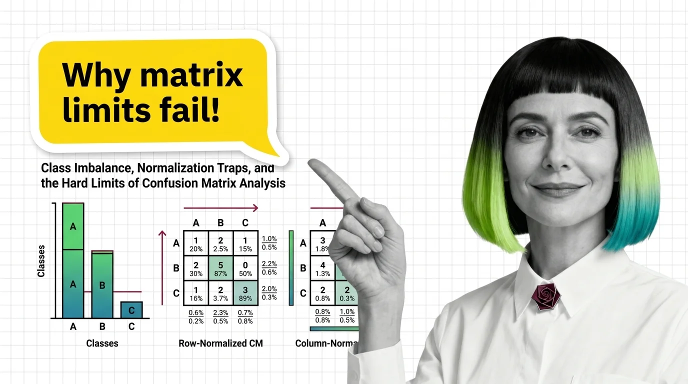
Table of Contents
ELI5
A confusion matrix counts a classifier’s correct and incorrect predictions in a grid. But when one class vastly outnumbers the other, the grid makes bad models look good — getting the majority right is trivially easy.
A classifier hits 90% accuracy on a medical screening task, and the team signs off. Months later, someone notices: it missed nearly every positive case. The Confusion Matrix was right there the whole time — four cells, clearly labeled. The problem was never visibility. It was which cell anyone bothered to read.
The Arithmetic of False Confidence
Most introductions to the confusion matrix present it as a clean accounting tool: true positives, true negatives, false positives, false negatives, arranged in a 2×2 grid. Count the cells, compute accuracy, move on. This framing works — until the class distribution stops being balanced, at which point the same grid becomes a mechanism for self-deception.
Why is a confusion matrix misleading with imbalanced datasets
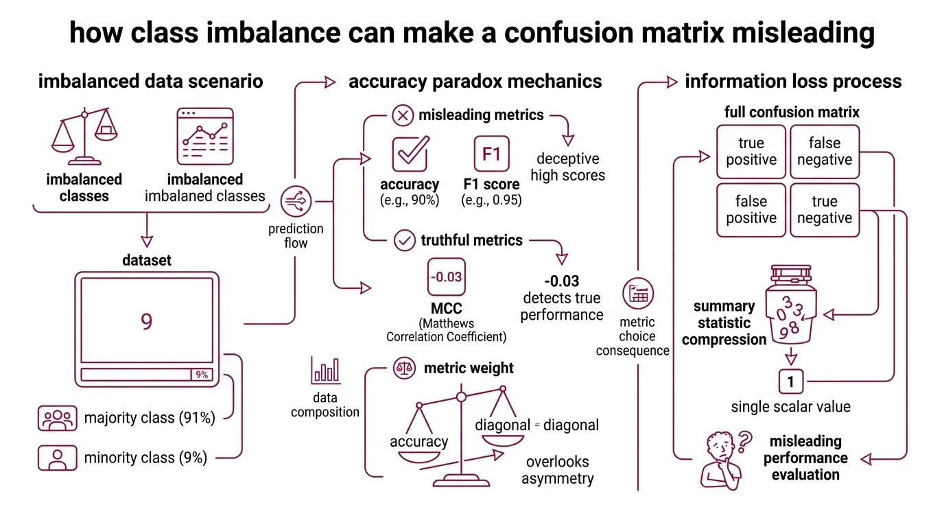
Consider a dataset where 91% of samples belong to the positive class. A model that predicts “positive” for every input — no learning, no feature extraction, pure default — achieves 90% accuracy. That number feels competent. The F1 score reinforces the illusion at 0.95. But the Matthews Correlation Coefficient tells a different story: MCC = −0.03, a value indistinguishable from random guessing (Chicco & Jurman).
This is the accuracy paradox, and it is not a theoretical curiosity. It is the default failure mode of any Binary Classification task where classes are skewed.
The mechanism is arithmetic, not statistical. Accuracy weights every correct prediction equally. When the overwhelming majority of samples belong to one class, correctly labeling those samples accounts for nearly all of the score — regardless of what the model does with the rest. The confusion matrix faithfully records all four cells, but accuracy reads only the diagonal and ignores the off-diagonal asymmetry.
The same grid, the same numbers. The metric chose to look at the wrong ones.
Class Imbalance does not corrupt the confusion matrix itself. It corrupts the summary statistics people extract from it. A model that never predicts the minority class will have a column of zeros on one side; the matrix shows this plainly. But the moment you compress four cells into a single scalar — accuracy, F1, even balanced accuracy — you lose resolution. The question is always which resolution you lost, and whether it matters for the task at hand.
Row Sums, Column Sums, and the Metrics They Erase
Normalization is where the confusion matrix becomes genuinely treacherous — not because the math is wrong, but because two different normalizations answer two different questions, and most practitioners never ask which question they need answered.
Difference between row-normalized and column-normalized confusion matrix
A raw confusion matrix reports counts. Normalization converts counts to proportions, but the denominator determines the meaning.
Row normalization (scikit-learn’s normalize='true') divides each cell by the row total — the actual number of samples in each class. The diagonal values become recall per class: of all the real positives, what fraction did the model catch? This is the clinician’s question. It answers: given that a patient is sick, how likely is the model to flag them?
Column normalization (normalize='pred') divides each cell by the column total — the number of predictions for each class. The diagonal values become precision per class: of everything the model labeled positive, what fraction actually was? This is the operations question. It answers: given that the model raised an alarm, how likely is it real?
The trap is subtle. A row-normalized matrix can show 0.95 on the diagonal for the majority class and 0.30 for the minority class — revealing a severe recall gap. The same model’s column-normalized matrix might show balanced precision for both classes, suggesting equilibrium where none exists. Neither view is wrong. Presenting only the column-normalized view obscures the very failure mode that class imbalance creates (scikit-learn Docs).
There is a third option: normalize='all', which divides every cell by the total sample count. This produces a joint probability table — useful for understanding global outcome distribution, but it compresses class-level performance into a single denominator that dilutes minority-class signals even further.
Not a bug. A design choice with consequences.
Beyond the Four-Cell Grid
The confusion matrix records outcomes at a single decision threshold. This is simultaneously its greatest strength — concrete, interpretable, auditable — and its most limiting structural constraint. Every cell in the grid is a snapshot of one operating point, frozen in place.
What are the limitations of using a confusion matrix as the only evaluation metric
Every confusion matrix is a photograph taken at one threshold. Move the decision boundary by 0.01, and every cell can shift. A model might look terrible at the default 0.5 cutoff but separate classes cleanly at 0.3. The matrix never shows this; it only reports the world where you set the cut.
This is why threshold-independent metrics exist. ROC curves plot true positive rate against false positive rate across all thresholds, making them especially useful for domains with skewed class distributions and unequal error costs (Fawcett). The Area Under the ROC Curve captures discriminative ability without committing to a single operating point. For imbalanced datasets, precision-recall curves often reveal more — a model with strong AUC-ROC can still have poor minority-class performance, visible only in the PR space.
The confusion matrix also carries a hidden assumption: all errors cost the same. A false negative in fraud detection — a missed fraudulent transaction — and a false positive — flagging a legitimate purchase — produce identical cells in the grid. But their operational consequences differ by orders of magnitude. The matrix provides no mechanism for encoding cost asymmetry; that interpretation lives entirely outside the grid.
For Model Evaluation beyond the binary case, the limitations compound. A multiclass confusion matrix grows as N×N, and summary metrics face the macro-vs-micro averaging problem. Macro averaging treats every class equally regardless of support; micro averaging weights by class frequency, which brings the imbalance problem right back. The Precision, Recall, and F1 Score are sensitive to class distribution in ways that the geometric mean of sensitivity and Specificity is not (Luque et al.).
The MCC — ranging from −1 through 0 to +1 — uses all four cells of the confusion matrix simultaneously and is argued to be preferred over accuracy and F1 for binary tasks (Chicco & Jurman). But even MCC reduces the matrix to a single number. Every scalar metric is a lossy compression. The question is always which information the compression discards.
When the Grid Stops Being Enough
If a model’s confusion matrix shows high recall for the minority class, the false positive cost may be worth absorbing — depending on the domain. If recall is low and precision is high, the model is conservative: it rarely raises false alarms but misses real cases. These are engineering trade-offs, not quality scores, and they require domain-specific cost reasoning to interpret.
The practical rules follow from the mechanism:
- If your dataset has a severe class ratio, accuracy is not a useful performance signal. Start with recall for the minority class and precision for the majority class; then evaluate the trade-off.
- If you are comparing models, pair the confusion matrix with a threshold-independent metric — AUC-ROC or AUC-PR — not instead of the matrix, but alongside it. The matrix tells you what happens at one operating point; the curve tells you what is possible.
- If you report a normalized confusion matrix, report both normalizations. Or report neither and use raw counts with class frequencies stated explicitly.
scikit-learn 1.8.0 introduced confusion_matrix_at_thresholds, which returns TP, FP, FN, and TN at each threshold in a single call (scikit-learn Changelog) — a step toward making threshold-dependent analysis the default rather than the afterthought.
Rule of thumb: If a single metric looks reassuring on imbalanced data, it is probably hiding the failure — not proving the model works.
When it breaks: The confusion matrix assumes discrete class assignments and a fixed threshold. For probabilistic outputs, calibration curves and proper scoring rules (Brier score, log loss) capture information the matrix structurally cannot — specifically, whether the model’s confidence is meaningful or decorative. The matrix also fails silently in the presence of Benchmark Contamination: a model that memorized the test set produces a perfect grid that reveals nothing about generalization.
The Data Says
The confusion matrix is not a diagnostic. It is a photograph of a diagnostic — taken from one angle, at one threshold, under one cost assumption. The grid itself is honest. The failures live in what people choose to compute from it, and what they choose to ignore.
AI-assisted content, human-reviewed. Images AI-generated. Editorial Standards · Our Editors