Beyond Transformers for Developers: What Maps and What Breaks
Table of Contents
Three weeks after your team shipped a 2026-generation model into staging, the cluster metrics told a contradictory story. The provisioning plan said roughly 1.5 terabytes of VRAM for a 671-billion-parameter model. The actual workload — once it started handling real traffic — showed three of your eight GPUs sitting near idle while two maxed out. Latency stayed inside the SLA. Cost per token did not. And none of the dashboards you had built for your Java services lit up with anything useful.
That incident is not a configuration bug. It is what you observe when a software developer’s mental model — shaped by stateless services, horizontal scaling, and deterministic routing — meets an architecture family where VRAM footprint and effective compute have been deliberately decoupled, where memory layout is megabyte-scale per request instead of kilobyte-per-token, and where “multimodal” is a scope word that names three components, not one.
This article is a map. Not of the full mechanism — the deep explainers carry that — but of where your existing engineering instincts still predict reality, and where they quietly stop. Four architecture families have pushed their way into production endpoints this year: mixture-of-experts, state space models, multimodal stacks, and the vision transformers that feed them. Each one rewards a different set of transfers from classical systems work, and each one breaks a different assumption you did not know you were making.
The 671-Billion Number That Isn’t Your Cluster Size
Start with the provisioning surprise. A Mixture Of Experts model carries a total parameter count — the number usually printed on the marketing page — and an active parameter count, which is what actually fires on any given token. For DeepSeek-V3 the split is stark: 671 billion total, 37 billion active per token, spread across 256 routed experts plus one shared expert per MoE layer (DeepSeek Technical Report). Mixtral 8x22B carries 141 billion total and 39 billion active. Llama 4 Maverick reaches 400 billion total on only 17 billion active, with 128 routed experts.
The capacity-planning instinct still applies. You still think in weights-to-VRAM ratios, you still care about batch sizing, and you still need to match precision to your hardware. But the coefficient you were multiplying by is wrong. VRAM footprint is governed by the total parameter count; inference FLOPs are governed by the active count. Provision for the first, bill against the second, and the two numbers are no longer coupled the way they were in dense models.
The mental model that breaks cleanly is “total parameter count equals model size equals hardware cost.” In a dense model it did. In an MoE model it does not — roughly 94% of DeepSeek-V3’s parameters are architecturally present but computationally silent on any given forward pass. If you sized the cluster against the headline number, you overpaid. If you sized against active parameters, your GPUs started thrashing as soon as the router balanced unevenly. For the full architecture, MONA’s prerequisites piece walks the building blocks; for the deployment contract, MAX’s open-weight MoE guide covers the hardware-mapping step explicitly.
When Your Load Balancer Instinct Actually Helps
Now the second surprise: one GPU at 100%, others at 30%. A senior backend developer reads that graph and reaches for a familiar diagnosis — broken routing, a hotspot key, an imbalanced shard. That instinct is correct in spirit and wrong in mechanism, and the difference matters.
Why VRAM Decouples From Active Compute
Inside an MoE layer, a small learned router assigns each token to a subset of experts — top-1 in Switch Transformer, top-2 in Mixtral, top-8 in DeepSeek-V3 with an auxiliary-loss-free bias term replacing the traditional load-balance penalty (DeepSeek Technical Report). The router is not configured. It is trained. And when training goes poorly, it learns to funnel most tokens to a favorite expert — a pattern the field calls routing collapse. Early and late transformer layers are especially prone to it, while middle layers tend to distribute more evenly (Cerebras Blog).
Your classical load-balancing intuition predicts the symptom correctly. It does not predict the fix. You cannot reweight the router the way you would re-hash a consistent-ring shard. The imbalance is encoded in the weights, and the standard mitigation is a load-balancing loss term applied during training that penalizes uneven utilization. At inference, you inherit whatever the trained router chose.
Which Software Instincts Predict MoE Behavior
The transfer that holds: fleet-thinking still works. Expert parallelism distributes experts across GPUs, and the communication pattern between them is all-to-all. At DeepSeek-V3 scale, NVIDIA measured communication overhead exceeding 50% of training time before targeted optimization (NVIDIA Hybrid-EP Blog). If you have ever debugged a microservice fleet where cross-pod chatter dominated CPU time, the shape is familiar.
The transfer that breaks: the assumption that adding more experts linearly adds capacity. It does not. Every expert must reside in GPU memory even though only a fraction activate per token. A model advertising “17 billion active parameters” may demand the VRAM footprint of a dense 45-billion-parameter model — Mixtral 8x7B requires approximately 90 GB in bfloat16 while only firing 13 billion parameters per forward pass (Friendli AI). Memory scales with total, not active. Plan for the first number, or the second GPU spike you see will not be a transient.
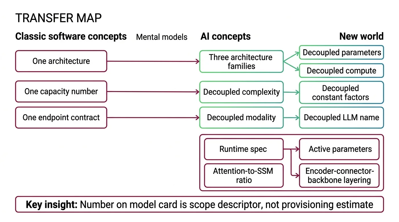
Mental Model Map: Beyond Transformers From: One architecture, one capacity number, one endpoint contract Shift: Three architecture families have decoupled parameter count from compute, complexity class from constant factors, and modality from the LLM that names it To: A runtime spec with active parameters, attention-to-SSM ratio, and encoder-connector-backbone layering Key insight: The number on the model card is a scope descriptor, not a provisioning estimate
Long Context Stopped Being a Transformer Problem
A different dashboard, a different surprise. Your long-context endpoint — a 256K-window model, advertised for document reasoning — runs at a fraction of the cost you modeled for, then becomes expensive in ways that have nothing to do with attention quadratics.
Why Linear-Time Intuition Misleads at Short Sequences
A State Space Model processes a sequence by carrying a compressed hidden state forward, updated token by token. Unlike self-attention, which scales quadratically with sequence length, a selective SSM runs in linear time. That fact launched a thousand blog posts and one valid intuition: at long enough sequences, SSMs win.
Not at every sequence length. Not by default. Under 8,000 tokens, transformers still run up to 1.9× faster in head-to-head comparisons; the crossover sits near 57,000 tokens, where SSMs reached up to 4× faster with roughly 64% less memory (SSM long-context paper). On edge GPUs, the custom kernels that make SSMs fast in theory become the dominant cost in practice — more than 55% of inference latency traced to those kernels in the same study, because their element-wise sequential nature resists the parallelism GPUs are built for.
Complexity class is not the whole story — constant factors are. Your instinct that “linear beats quadratic” is asymptotically correct and practically wrong for the short-prompt workloads most production systems actually run. It also misses the architectural reality of 2026: almost nothing in production is pure SSM. Jamba 1.5 pairs one attention layer per eight total with a Mamba-MoE backbone at 256K context (AI21 Blog). NVIDIA’s Nemotron-H-56B stacks 54 Mamba-2 layers, 54 MLP layers, and only 10 self-attention layers (NVIDIA ADLR). The architecture question is not attention versus SSM. It is how much of each, in what configuration, for which workload.
Not a failure of the SSM idea. A recalibration of where the idea pays.
The deeper surprise is memory layout. An attention layer stores a KV cache that grows per token in small kilobyte increments. An SSM layer stores a fixed-size state measured in megabytes and overwritten in place as tokens arrive. Standard prefix caching — the technique that lets a serving system reuse prior prompt computations across requests — works for attention KV cache because the cache is additive and replayable. It fails for SSM layers because the state has been written over; there is no prefix to reuse (SGLang hybrid support). If your serving stack depends on prefix caching for cost control, a hybrid SSM-attention model will silently break that assumption. For the structural tax and its second-order effects, MONA’s hard-limits piece traces the compression problem end to end.
Multimodal Is Three Layers Sharing One Endpoint
The third pattern is the most misread. A model card says “natively multimodal.” A developer hears: the language model looks at the image. The language model, as a rule, does not look at anything.
Why “Native Multimodal” Doesn’t Mean Pixels
A Multimodal Architecture in 2026 is converging on a single pattern: specialist encoders compress raw signals — pixels, waveforms — into feature vectors, a lightweight connector projects those features into the language model’s token space, and a shared LLM backbone does the actual reasoning over a mixed token stream (Zhang et al., MM-LLMs survey). The variety lives in the connector — projection-style (a small MLP, as in LLaVA), query-based (BLIP-2’s Q-Former, Flamingo’s Perceiver Resampler), or fusion-based cross-attention — not in the backbone.
“Native multimodal” means the model was pre-trained on interleaved multimodal sequences rather than text-first-then-image-bolted-on. It does not mean the LLM perceives images. It means the failure surface now spans three components, each with its own contract.
| Layer | Owns | Typical Failure |
|---|---|---|
| Modality encoder | Resolution, patch size, feature dimension | Silent resolution downgrade on variable-aspect inputs |
| Connector | Shape of the vision-to-language projection | Grounding decay as output length grows |
| LLM backbone | Token-space reasoning, generation | Hallucinated content that ignores the visual evidence |
A Vision Transformer like SigLIP 2 produces patch embeddings. The connector turns those into a fixed number of tokens — LLaVA-OneVision pools video to 196 tokens per frame (LLaVA-OneVision paper). The backbone generates text. When your debugging instinct says “the model hallucinated,” you need to know which layer betrayed the contract. Encoder hallucination is different from connector bandwidth loss, which is different from backbone drift. MAX’s pipeline guide walks the three-layer contract explicitly; MONA’s prerequisites piece covers the modality-gap geometry that explains why retrieval quality breaks even when ingestion works.
Which Marketing Phrases Cost You the Most Incidents
Three vendor framings account for the largest share of misprovisioned launches in 2026, and each one survives because it maps onto an older intuition that no longer predicts the new behavior.
“Trillion-parameter model” is the first. In a dense world, parameter count was a usable proxy for compute, for memory, and for latency. In an MoE world, those three numbers have decoupled. The only provisioning question that matters is the active count and the expert routing topology — if you cannot state both for your chosen model, you are guessing. Mixtral 8x22B’s 141B total is not a 141B workload. Llama 4 Maverick’s 400B is not a 400B workload. Plan to the active number, budget VRAM to the total, and know which is which.
“Linear-time state space model” is the second. The linear-time claim is correct at the asymptote and misleading at the sequence lengths most production systems actually run. Pure Mamba rarely ships. Hybrid SSM-attention models are the 2026 default for 256K-and-above workloads, and the serving-stack complexity they introduce — SSM state layout, prefix-caching incompatibility, hybrid-aware kernels — is not optional (SGLang hybrid support). Adopt the architecture, budget the serving work.
“Native multimodal” is the third. It means pre-trained on interleaved sequences. It does not mean the language model sees pixels, and the three-layer stack is still present under the API. When grounding fails, it fails in one of three places, and the debugging path depends on which one. “Just add more experts to scale capacity” — or “scale Mamba the way you scale a transformer” — are the systems-engineering reflexes that carry the day-one assumptions of older architectures into systems that were deliberately designed to break them.
Your runtime spec needs the active parameter count, the attention-to-SSM ratio, and the encoder-connector-backbone contract. The vendor datasheet alone will not give you all three.
The Runtime Contract You Now Need
Total parameter count, sequence-length complexity, and the word “multimodal” are all scope descriptors, not architectural specifications. Treat them as starting points for a runtime contract, not as capacity estimates. For the three-box map through this cluster, begin with the state space model explainer, the MoE definition, and the multimodal architecture walkthrough.
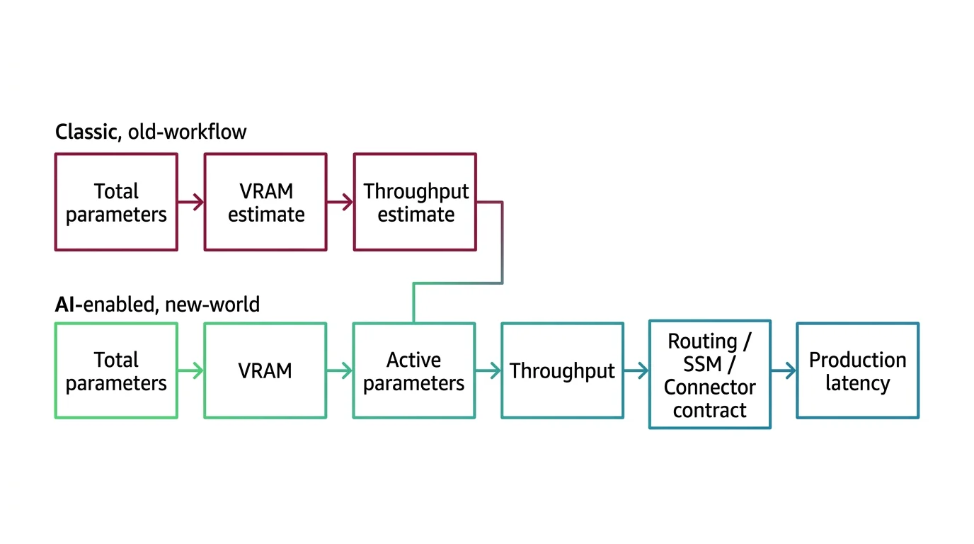
Shift Diagram: Provisioning a 2026 model endpoint Classic: Total parameters → VRAM estimate → throughput estimate AI: Total parameters → VRAM → Active parameters → throughput → Routing / SSM / connector contract → production latency
These three families are not variants of the transformer contract. They are three different contracts the transformer used to hide, each with its own provisioning row: active parameters, attention-to-SSM ratio, and encoder-connector-backbone layout. Add them to your capacity plan before the next long-prompt incident adds them for you — MAX’s open-weight MoE guide walks the deployment mechanics end to end.
FAQ
Q: Do I need to understand MoE, state space models, and multimodal architectures to use their APIs?
A: You do not need to build them, but you need the contracts: active parameter count for MoE provisioning, attention-to-SSM ratio for long-context serving, and encoder-connector-backbone layering for multimodal debugging. Without those, production surprises read as random.
Q: What is the difference between total and active parameters in mixture-of-experts models?
A: Total parameters are what you load into VRAM; active parameters are what fire per token. DeepSeek-V3 holds 671 billion total and activates 37 billion per token (DeepSeek Technical Report). Memory scales with total; inference FLOPs scale with active.
Q: Why do hybrid SSM-attention models break standard prefix caching?
A: An attention KV cache is additive and replayable. An SSM state is fixed-size and overwritten in place as tokens arrive, so there is no prefix to reuse (SGLang hybrid support). Serving stacks that rely on prefix caching need hybrid-aware kernels to retain long-context throughput.
AI-assisted content, human-reviewed. Images AI-generated. Editorial Standards · Our Editors