The Architecture Name on the Spec Sheet Is a Failure Contract
You wired a vendor’s image upscaler into your product pipeline — an off-the-shelf model, a few lines against its API, sharper resolution on demand. It worked in the demo. Then the batch ran, and a slice of the results came back wearing the same invented texture: the same smeared grain stamped across a hundred different product photos. You swapped the weights, adjusted the input size, fed it cleaner source images. The artifact held its ground. No knob you owned could move it, because the failure was never in your integration. The model card said one thing about the architecture underneath: GAN. That word was a contract — and the clause you had triggered was mode collapse.
An architecture family name on a model card — convolutional, recurrent, adversarial, graph — is not an implementation detail hidden behind the interface. It is a capability envelope: it fixes what a model can represent and how it fails. The crack in your classical mental model is the assumption that two models with the same benchmark score are interchangeable components. They are not — and the difference is the failure mode the benchmark never printed.
Why Your Database Instinct Still Applies
You already choose infrastructure by the access pattern it makes cheap or impossible, not by a single headline number.
You do not pick a datastore on throughput alone. You pick it on what it makes cheap — B-tree range scans, key lookups — and what it makes painful, like graph traversal bolted onto a relational store. Reading a library’s complexity contract before you adopt it is the same reflex: you want the Big-O before you build on the call. That instinct transfers cleanly here. A Convolutional Neural Network is built around a spatial-locality prior — it makes detecting local, reusable patterns cheap, and it makes global, long-range relationships across an image expensive to see. A Recurrent Neural Network makes streaming, one-step-at-a-time memory cheap, and lets long-distance dependencies decay. Each family is a set of access patterns for representation.
The transfer is real, but it is shallower than the vocabulary suggests. When you migrate a database, you own the switch. When you call a hosted model, the vendor owns the architecture, and your only lever is whether you adopt it. So the instinct to read the cost contract first matters more here, not less — because you read it once, at adoption, and then you live with it. The pattern that a deep CNN’s receptive field may never reach far enough for global structure is not a tuning detail; it is the boundary in the geometry of the architecture itself, documented long before your image reaches it.
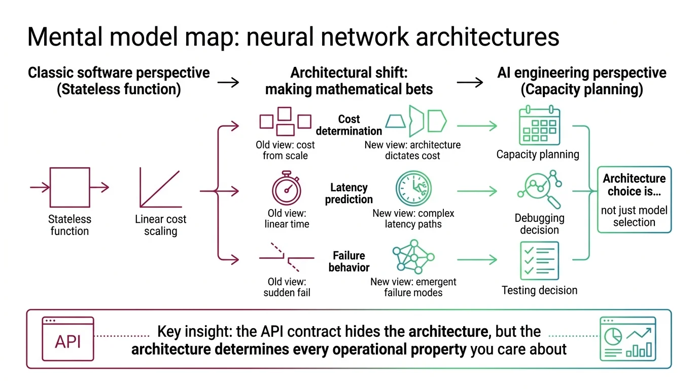
Mental Model Map: neural network architecture families From: the architecture name is an implementation detail behind the API Shift: the name is the access-pattern contract for representation To: pick the family by the failure it makes cheap to avoid Key insight: choosing an architecture family is choosing a data structure — you are selecting what is cheap to represent and what is structurally hard to reach.
The Benchmark Hides the Failure Mode
Two models can post the same accuracy and still commit you to entirely different ways of breaking.
A convolutional backbone and a vision transformer can land within a point of each other on a top-1 leaderboard, yet the convolutional model cannot reach across the whole image the way attention does, and the transformer needs far more pre-training data to reach that score at all. A Generative Adversarial Network and a diffusion model can produce comparable perceived quality, but the adversarial network generates in a single fast pass and can collapse to one output, while the diffusion model is stable and slow. The benchmark measures the average case on a curated set. The failure mode lives in the tail your users generate — and the tail is exactly what the leaderboard trims.
Think about what an accuracy score actually samples. A vision benchmark scores a model on a fixed, balanced test set assembled by researchers. Your users send a different distribution — odd lighting, rare classes, inputs no benchmark curator anticipated. A convolutional model and a transformer that tie on the curated set can diverge sharply on that traffic, because each family’s blind spot is a different shape. One misses the global relationship across the frame; the other never saw enough of your edge case to generalize to it.
In practice, a benchmark number tells you how a model does on the data someone else chose. It says nothing about which family-specific failure will surface on yours, and that is the number your incident review will actually care about.
Each Family Ships Its Own Breakage
Every architecture family carries a signature failure that no version bump removes, because the failure is a property of the math, not a bug in the release.
Mode collapse in a GAN is not a defect awaiting a patch — it is a structural consequence of the minimax game between generator and discriminator, the gap between a theoretical equilibrium and the finite networks that must approximate it. Memory decay in a recurrent network is not a training accident; it is a property of repeated matrix multiplication, where the gradient shrinks exponentially across long sequences. Oversmoothing in a Graph Neural Network is the same story in a different geometry: each message-passing round averages a node with its neighbors until every node looks the same, so stacking depth destroys the distinctions that made the model useful. None of these is a line you can find and fix.
| Family | What it makes cheap | The structural failure you inherit |
|---|---|---|
| CNN | local spatial features, few parameters | global, long-range context (a receptive-field ceiling) |
| RNN / LSTM | streaming, sequential memory | long-distance dependency decay |
| GAN | single-pass, real-time generation | mode collapse and training instability |
| GNN | relational, graph-shaped reasoning | oversmoothing and neighbor explosion at scale |
| Variational Autoencoder | a smooth, navigable latent space | blurry reconstructions — the pixel tax of the loss function |
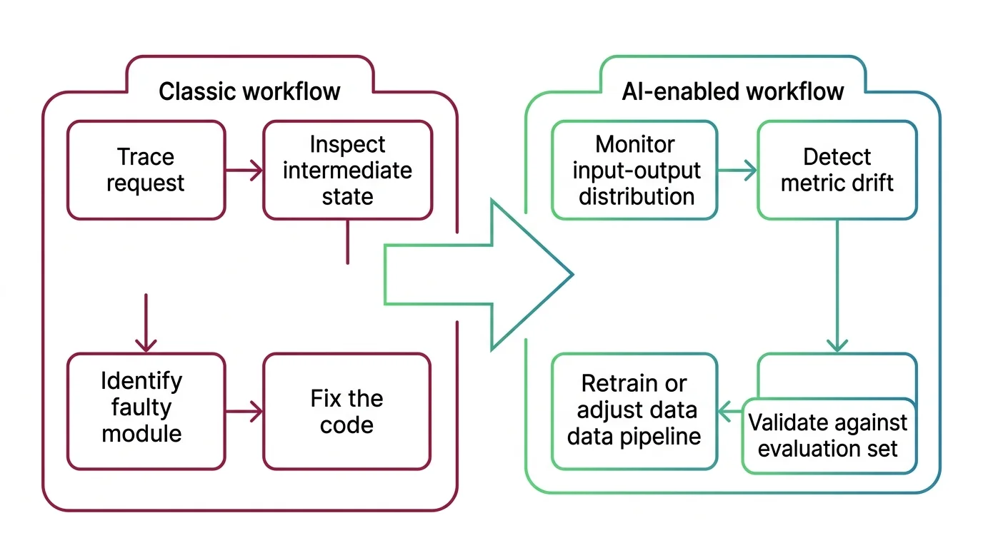
Shift Diagram: adopting a model by architecture family Classic: match the API → compare one benchmark → swap components freely AI: match the API → inherit the family’s failure mode → redesign, not swap, to change it
The practical consequence is that these failures do not raise exceptions. They degrade output quality in ways your logs will not flag, so the family you picked decides which silent failure you now have to monitor for.
The Name Is Not an Implementation Detail
The dangerous move is reading the architecture name the way you read whether a library uses a red-black tree or a hash map — as a private internal you are entitled to ignore.
When you call map.get(key), the balancing of that tree is genuinely sealed off. The contract is the complexity bound and the return value; you never feel the internals, and you are right not to care. An architecture family does not stay sealed. Its internals leak through the interface into the behavior your users see — the collapsed texture, the forgotten early token, the blurred reconstruction. Not a leaky abstraction you can patch. A capability ceiling no prompt or fine-tune moves.
There is a second leak, and it runs the other way. Because the vendor owns the model, they can retrain it, re-tune it, or swap the checkpoint — and the output distribution can shift underneath you while the API signature stays byte-for-byte identical. You get a behavior change with no version bump to blame. In practice, this means the architecture name is the one part of the contract you must scope at adoption time, because it is the part you can never patch at call time.
Bigger Does Not Mean the Old One Left
The last assumption to drop is that a newer, larger family cleanly supersedes the one before it.
The spec sheet increasingly refuses that story. Production vision systems now fuse convolutional backbones with transformer layers rather than choosing between them — CNNs extract local patterns while attention handles global dependencies, and the hybrid wins the production races that a pure architecture used to. Older families specialize instead of disappearing: as of 2026, GANs have largely ceded quality-first image generation to diffusion but still hold the latency-critical ground where a single fast pass beats iterative denoising. And recurrence, long declared dead, is finding its way back in new forms — xLSTM and state-space designs like Mamba trade quadratic attention cost for linear-time sequence modeling, though several of their headline speedups are still vendor-reported and await independent replication.
The label on next year’s model card is likely to be a compound, and each half contributes its own cheap operations and its own breakage. For the full prerequisite map and the questions a model card raises, see the topic hub. Read a hybrid the way you would read a struct made of two data structures: not as a single new thing, but as the sum of what each part makes fast and what each part makes fragile.
Before You Adopt That Model Card
The gap between a well-written explainer and a decision tool is a checklist you run against your own stack. These are the questions to answer before the integration, not after the incident.
| Runtime question | Why it matters |
|---|---|
| What does this family make structurally expensive? | That is where your tail failures cluster — never where the benchmark looked. |
| What is this family’s signature failure, and can I detect it in production? | Mode collapse, memory decay, and oversmoothing raise no exceptions; you need a metric or you are blind to them. |
| If the vendor retrains, what stays fixed? | The API signature can hold while the output distribution moves; the envelope is the part that will not. |
| Is this one family or a hybrid? | Each half contributes its own cheap operations and its own breakage — scope both. |
| Can I change this failure by prompting or fine-tuning? | If not, the fix is architectural, and it has to be a decision you make before you depend on the model. |
An architecture family is a data structure for representation: it makes some things cheap, some things impossible, and one thing inevitable — its own failure mode. Read the name on the model card the way you read a complexity contract, before you build on it. Then open the deep article for whichever family you are inheriting, and scope the failure while it is still a design decision instead of a production incident.
AI-assisted content, human-reviewed. Images AI-generated. Editorial Standards · Our Editors