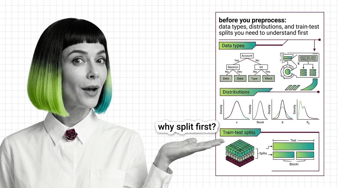
Before You Preprocess: Data Types, Distributions, and Train-Test Splits You Need to Understand First

A model scores 0.98 on validation. Everyone celebrates. Then it goes live and the accuracy collapses to something barely better than a coin flip. Nothing in the code changed. The model didn’t degrade — it was never that good. The validation score was borrowing from the future, and nobody noticed because the leak happened before a single line of modeling code ran.

This is the most common way a Data Preprocessing pipeline lies to you, and it almost always traces back to decisions made before preprocessing even began. The order of operations matters more than the operations themselves.

The Three Things You Inspect Before You Transform Anything

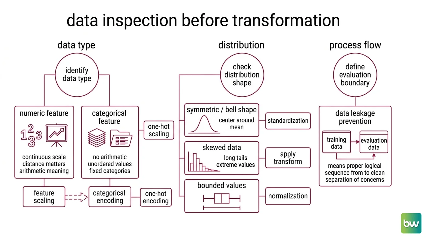
Preprocessing is not the first step. Inspection is. Before you scale, encode, or impute, you need a mental model of what the data actually is — because every transform you apply is a bet about the structure underneath it. Pick the wrong transform for the wrong data type and you don’t get an error; you get a model that trains fine and reasons badly.

What do you need to know before preprocessing data for machine learning?

Three properties decide every preprocessing choice you’ll make: the data type of each feature, the distribution of its values, and the boundary between training and evaluation.

Start with data type, because it determines the entire branch of transforms available to you. A numeric feature — age, price, temperature — lives on a continuous scale where distance means something; the gap between 10 and 20 is the same as between 50 and 60. A categorical feature — country, product class, blood type — has no such arithmetic. “Germany minus France” is not a number. Feed raw category labels into a model that assumes numeric distance and it will invent an ordering that doesn’t exist. This is why numeric features route toward Feature Scaling and categorical ones toward Categorical Encoding, often One Hot Encoding, which expands each category into its own binary column so no false ranking sneaks in.

Then comes distribution — and here I mean the practical shape of the values, not probability theory. Are they roughly symmetric around a center, or skewed with a long tail? What’s the scale — single digits, or millions? Are there extreme values sitting far from everything else? The shape dictates the transform. A symmetric, bell-like feature responds well to Standardization, which removes the mean and rescales to unit variance. A bounded feature might prefer Normalization into a fixed range. A heavily skewed feature often needs a log transform first, or the scaler will be dragged around by its tail. And before any of that, you check for Outlier Detection, because a single absurd value can distort the mean and standard deviation that scaling depends on.

The third property is the one people skip: the split. You need to decide where training data ends and evaluation data begins before you compute anything from the data — and the next section is where that turns from housekeeping into the difference between a real score and a fictional one.

Why does inspecting the distribution change which transform you pick?

A transform is a function fitted to the data it sees. Standardization computes a mean and a standard deviation, then subtracts and divides. Normalization finds a minimum and maximum, then squeezes everything between them. Missing Data Imputation computes a fill value — a mean, a median, a most-frequent category — from the column.

Notice what every one of these has in common: each transform learns a parameter from the data. The scaler’s mean is learned. The encoder’s category set is learned. The imputer’s fill value is learned. And the moment a transform learns something, the question becomes unavoidable: learned from which data?

Get that question wrong and the transform leaks.

Why the Split Has to Come First

Here is the rule that reorders everything: you split before you preprocess. Not after you’ve cleaned the data, not after you’ve scaled it — first, before any transform touches a single value. The official scikit-learn guidance is blunt about it: always split the data into train and test subsets first, particularly before any preprocessing steps (scikit-learn Docs).

The reason is mechanical, not stylistic.

Why do you need to split data into train and test sets before preprocessing?

Imagine you standardize first. You take the full dataset, compute the mean and standard deviation across every row, and rescale. Then you split into train and test. It feels harmless — you only computed a mean. But that mean was calculated using the test rows. The scaling parameters now encode information about data the model is supposed to never have seen. When you evaluate on the test set, the test set is being measured against statistics it helped define.

That is the textbook definition of Data Leakage: using information at model-building time that would not be available at prediction time, which produces overly optimistic evaluation scores and poor performance once the model meets genuinely new data (scikit-learn Docs). The 0.98 from the opening was real arithmetic. It was just answering a different question than the one you thought you asked.

The fix is an ordering and a discipline:

• Split first. Carve out the test set before computing anything.
• Fit on training data only. The scaler’s mean, the encoder’s categories, the imputer’s fill value — all learned exclusively from the training rows. As the documentation puts it, the normalization mean must be the train mean, not the all-data mean (scikit-learn Docs).
• Transform the test set using the training parameters. You call fit (or fit_transform) on train, and only transform on test — never fit again. The test set gets reshaped by numbers it had no part in producing.

This is why train_test_split in scikit-learn is the gatekeeper of the whole pipeline. Its default holds out 25% of the data for testing when you specify neither a test nor train size (scikit-learn Docs). Pass random_state an integer and the split becomes reproducible — the same rows land in the same subset every run, which matters when you’re trying to tell whether a change to your model helped or whether you just got a luckier shuffle. And when your target classes are imbalanced, stratify=y preserves the class proportions across both subsets so your test set isn’t accidentally missing a rare class entirely.

The cleanest defense against leakage is to stop doing the bookkeeping by hand. A scikit-learn Pipeline binds the transforms to the model so that fit runs on the training fold and transform runs on validation and test automatically — the right method on the right subset, enforced by structure rather than memory (scikit-learn Docs). The leak doesn’t get caught; it never gets the chance to happen.

What Getting the Order Right Predicts

Once you internalize that every transform learns a parameter, the failure modes become predictable rather than mysterious.

• If your validation score is far higher than production performance and nothing in the model explains the gap, suspect that a transform was fitted on data including the test set.
• If you scaled before splitting, expect the inflation to shrink as your dataset grows — with more rows, the all-data mean and the train-only mean converge, so the leak gets quieter and harder to spot. Small datasets leak loudly; large ones leak silently.
• If your imputation fill value was computed across the whole dataset, your test set’s missing values are being filled with knowledge of the test set’s own distribution.

Understanding this also reframes Feature Engineering: any feature you derive from aggregate statistics — a column normalized by a global average, a count computed across all rows — is a transform too, and it leaks under exactly the same rules. The split has to come before the engineering, not just before the scaling.

Rule of thumb: If a step computes anything from the data, fit it on training rows only and apply it everywhere else with transform.

When it breaks: Splitting first protects you from leakage introduced by your preprocessing, but it does not protect you from leakage baked into the features themselves — a column that secretly encodes the target, or time-series data where a random split lets the model train on the future and test on the past. For temporal data, a random Train Test Split is itself a leak; you need a chronological split instead.

The Tooling Has Quietly Changed Underneath You

One practical note, because the libraries you reach for have shifted. The Pandas 3.0 series made a dedicated string dtype and Copy-on-Write the defaults (pandas Blog), which means older tutorials demonstrating object-string columns and chained-assignment tricks describe behavior that no longer holds. The preprocessing concepts here are version-independent — a mean leaks the same way it did a decade ago — but the code you copy from a 2021 blog post may not run the way it reads.

The Data Says

Preprocessing decisions are downstream of three facts you establish first: the type of each feature, the shape of its distribution, and the line between train and test. Get the split wrong and every score afterward is fiction — not because the model is bad, but because the evaluation quietly measured the data against itself. Fit on train, transform on test, and let a pipeline enforce it.