Backpropagation Through Time, Vanishing Gradients, and Why Transformers Replaced Recurrent Networks

A recurrent neural network trained on a 200-word paragraph can track the subject of a sentence. The same architecture, given a 500-word paragraph, starts confusing that subject with a noun from three sentences earlier. The input grew longer — and the model grew worse. That degradation is not a bug in any particular implementation; it is baked into the arithmetic of how recurrence learns.

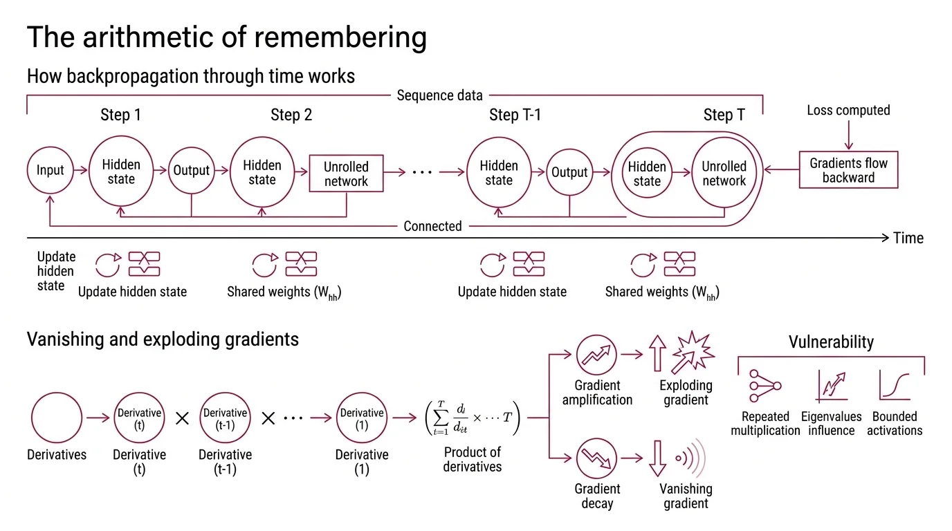
The Arithmetic of Remembering

Recurrent Neural Network architectures share a single weight matrix across every time step in a sequence. That sharing is the source of their elegance — and their central vulnerability. To see why, you need to follow the error signal as it travels backward through the unrolled computation graph.

How does backpropagation through time work in recurrent neural networks?

Backpropagation Through Time takes a familiar idea — standard Backpropagation — and stretches it across the time dimension. The network processes a sequence one token at a time, updating a Hidden State at each step. During training, the entire sequence is “unrolled” into what looks like a very deep feedforward network: one layer per time step, all layers sharing the same weights.

The loss is computed at the output, and gradients flow backward through every time step. At each step, the gradient passes through the same recurrent weight matrix W_hh and through the derivative of the activation function. The critical detail: because the weights are shared, the gradient reaching time step t depends on the product of those derivatives across every step from the output back to t. For a sequence of length T, the gradient arriving at step 1 involves T-1 repeated multiplications.

Werbos formalized this unrolling procedure in 1990, laying the mathematical foundation for training recurrent networks (Werbos (1990)). The algorithm is elegant. But repeated multiplication is either amplification or decay — and there is almost no stable middle ground.

When the Signal Decays to Noise

The gradient chain in BPTT is not inherently unstable. It becomes unstable because of what gets multiplied. The eigenvalues of the recurrent weight matrix and the bounded derivatives of activation functions conspire to either crush or amplify the learning signal — and for most practical sequences, crushing wins.

What causes vanishing and exploding gradients in RNNs?

The gradient flowing from time step T back to time step t is proportional to a product of terms, each containing W_hh and the activation derivative. If the largest eigenvalue of W_hh is less than 1, the product shrinks exponentially with distance. If it exceeds 1, the product grows without bound (D2L).

Sigmoid activation functions compound the decay. The derivative of a sigmoid is bounded between 0 and 0.25 — meaning every step in the chain multiplies the gradient by at most one-quarter. Over even a moderate number of steps, this compounding reduces the signal to numerical insignificance; the gradient does not fade gradually so much as collapse.

The Vanishing Gradient problem was formally identified by Hochreiter in his 1991 diploma thesis and independently demonstrated by Bengio et al. in 1994 (Hochreiter (1991) / Bengio et al. (1994)). The practical consequence is stark: a standard RNN struggles to learn dependencies beyond short spans. Information from the opening of a paragraph is invisible to the gradient by the time it reaches the final word.

Not a training failure. A structural limit.

Truncated BPTT offers a partial workaround — breaking the sequence into fixed-length windows and backpropagating only within each (D2L). It trades gradient accuracy for numerical stability, but it also caps the network’s ability to learn long-range patterns. The truncation window becomes a hard ceiling on memory.

Sequential by Design, Slow by Necessity

Even if you solve the gradient problem, recurrence carries a second constraint that no gating mechanism can remove. The sequential dependency that gives RNNs their temporal structure is also the bottleneck that prevents them from saturating modern hardware. Unlike Convolutional Neural Network architectures, which process spatial dimensions in parallel because each filter operates independently, RNNs offer no such escape.

Why can’t RNNs process long sequences or parallelize training like transformers?

A recurrent network computes hidden state h_t as a function of h_{t-1} and the current input. That dependency is strict: you cannot compute h_50 without first computing h_1 through h_49. The entire sequence must be processed in order, one step at a time — O(n) sequential operations for a sequence of length n.

On a GPU designed to execute thousands of operations simultaneously, most of the silicon sits idle, waiting.

Self-attention, introduced by Vaswani et al. in 2017, dissolves this dependency. Every position attends to every other position in a single parallel computation — O(1) sequential operations, regardless of sequence length. The original Transformer achieved 28.4 BLEU on WMT 2014 English-to-German translation (Vaswani et al. (2017)), but the benchmark score was almost secondary to the architectural insight: recurrence is not required for sequence modeling.

The cost of self-attention is quadratic in sequence length — O(n^2) memory and computation — which creates its own scaling problems for very long sequences. But the ability to saturate modern GPUs during training changed the economics of Neural Network Basics for LLMs research. Training runs that took weeks on recurrent architectures took days on Transformers, not because the math was simpler, but because the math was parallel.

The Gate That Bought Recurrence Three Decades

Long before self-attention, a different solution to the vanishing gradient problem kept recurrence relevant. Long Short-Term Memory — introduced by Hochreiter & Schmidhuber in 1997 — added a separate memory cell with a constant error flow, protected by learned gates that control what information enters, persists, and leaves (Hochreiter & Schmidhuber (1997)).

The original LSTM paper demonstrated learning across time lags exceeding 1,000 discrete steps, something standard RNNs could not approach. The constant error carousel — the unbroken pathway through the cell state — prevents gradient decay by maintaining a gradient of exactly 1 along the cell’s self-connection. The forget gate, input gate, and output gate learn which signals to preserve and which to discard, turning memory management into a trainable operation rather than a structural accident.

LSTM and its later variant GRU powered machine translation, speech recognition, and language modeling from the late 1990s through the mid-2010s. They did not eliminate the sequential bottleneck — every hidden state still depended on the previous one — but they extended the effective memory range enough to make recurrent networks practical.

The architecture’s lineage is not finished. xLSTM, introduced by Beck et al. in 2024, adds exponential gating and matrix memory to the LSTM framework. The authors report considerably faster training speeds than equivalently sized Transformers — though independent large-scale replication of those claims has not yet been published (Beck et al. (2024)). State space models represent a parallel lineage, blending recurrent-style sequential processing with sub-quadratic attention costs. As of 2025, hybrid architectures combining attention layers with recurrent or SSM layers are an active area of research; the field appears to be converging on mixed designs rather than betting on a single paradigm.

When it breaks: LSTM gates solve vanishing gradients but cannot solve the sequential bottleneck. For tasks requiring both long context and fast training — modern language models routinely process thousands of tokens — the O(n) sequential dependency makes pure recurrent architectures impractical regardless of gating.

Rule of thumb: If your sequence is short and your latency budget matters more than training throughput, recurrent architectures remain viable and memory-efficient. Once sequences grow long enough that gradient coverage or parallelism becomes the constraint, the math favors attention.

The Data Says

Recurrence failed at scale not because the idea was wrong, but because the arithmetic was unforgiving — gradients that decay exponentially cannot carry information across long sequences, and sequential computation cannot fill a GPU. Self-attention solved both problems simultaneously, at the cost of quadratic memory. The story is not over: gated recurrence, in new forms, is finding its way back into hybrid architectures that try to keep the strengths of both paradigms without inheriting either’s worst constraint.